User Guide
Everything you need to know about using SunTrace3D to analyze solar potential, simulate shadows, and estimate energy yield for any location worldwide.
View as Markdown (machine-readable)Video Tutorials
3D Solar Simulation Software Demo
Ground Mount Solar Farm — Full Engineering Walkthrough
Solar CRM Demo: Territory Scanning, 3D Roof Analysis & Direct Mail in 60 Seconds
How Architects Collect Client Feedback Directly on a 3D Model
Draw a Building on an Empty Lot and Design Its Solar in 40 Seconds
Test-Fit a Development Site in 60 Seconds — Site Planning
Your Solar Panels vs This Week's Weather — SunTrace3D Weather Forecast
SunTrace3D for Homeowners
SunTrace3D for Garden & Landscape
Your Solar Week, Before It Happens — The Weekly Forecast on Your Phone
SunTrace3D is a browser-based 3D solar analysis tool. No installation, plugins, or sign-up is required to get started. Simply open the viewer and explore.
Open the Viewer
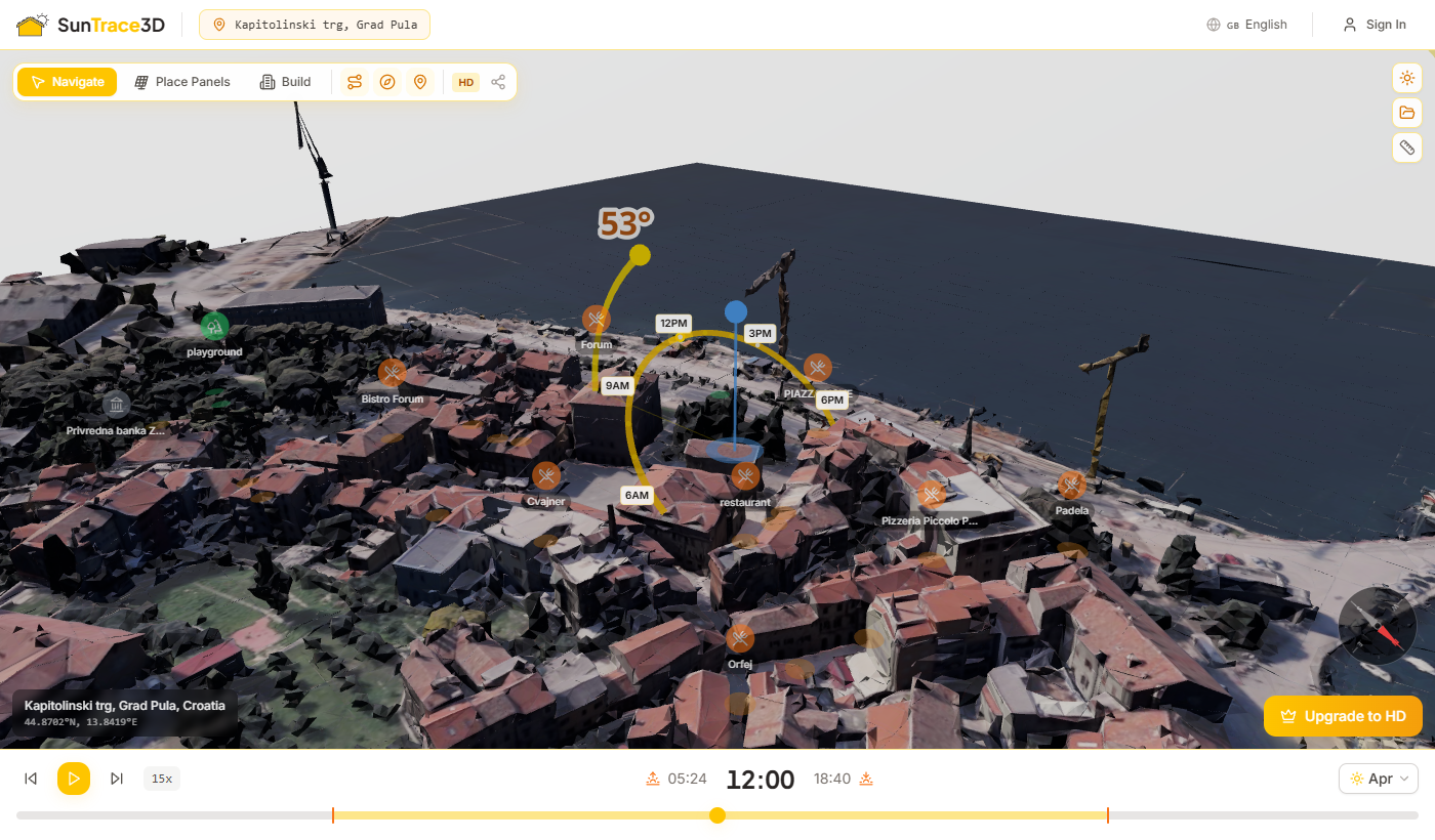
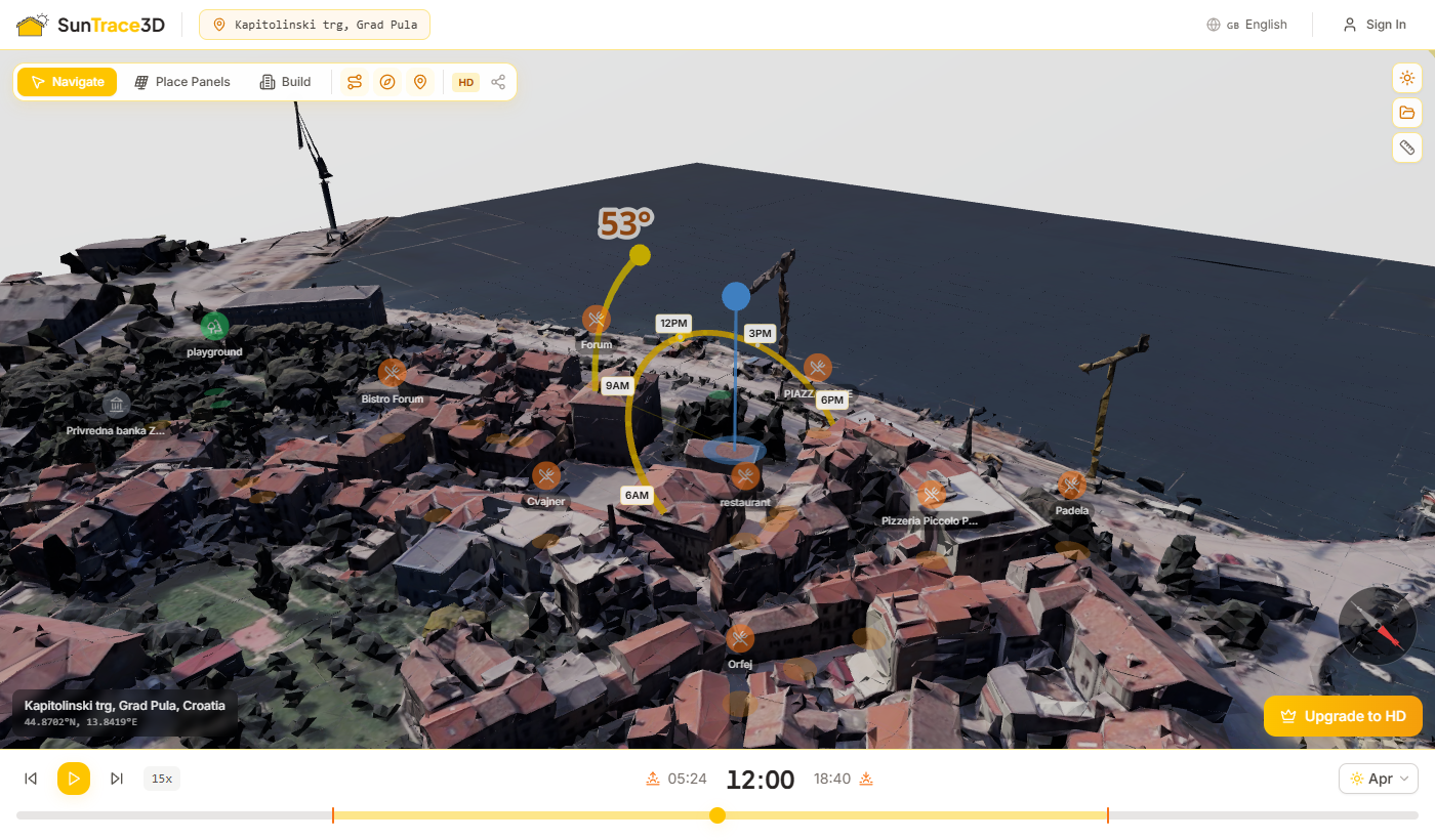
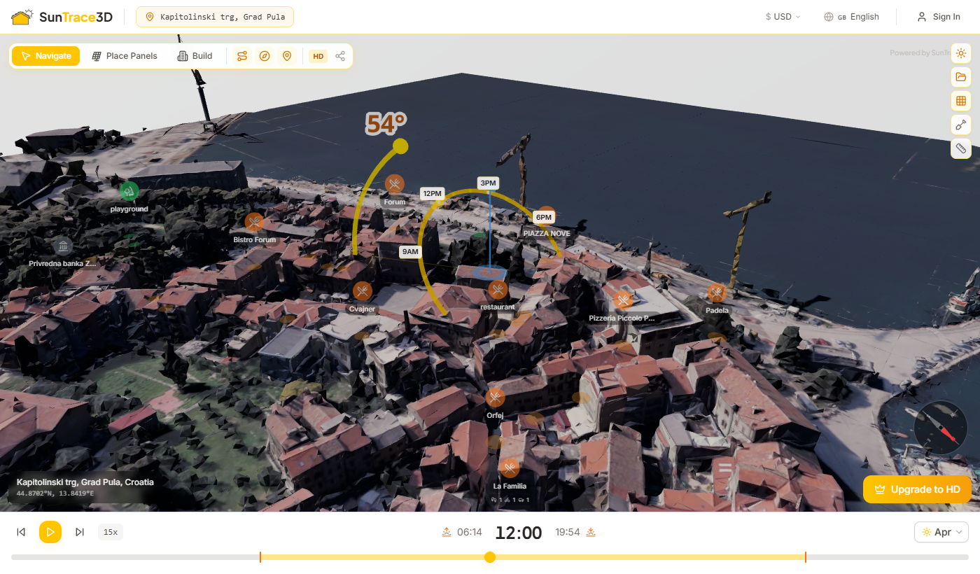
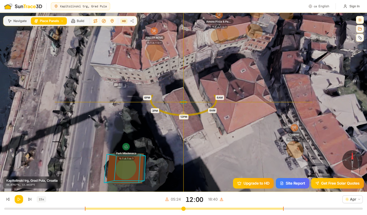
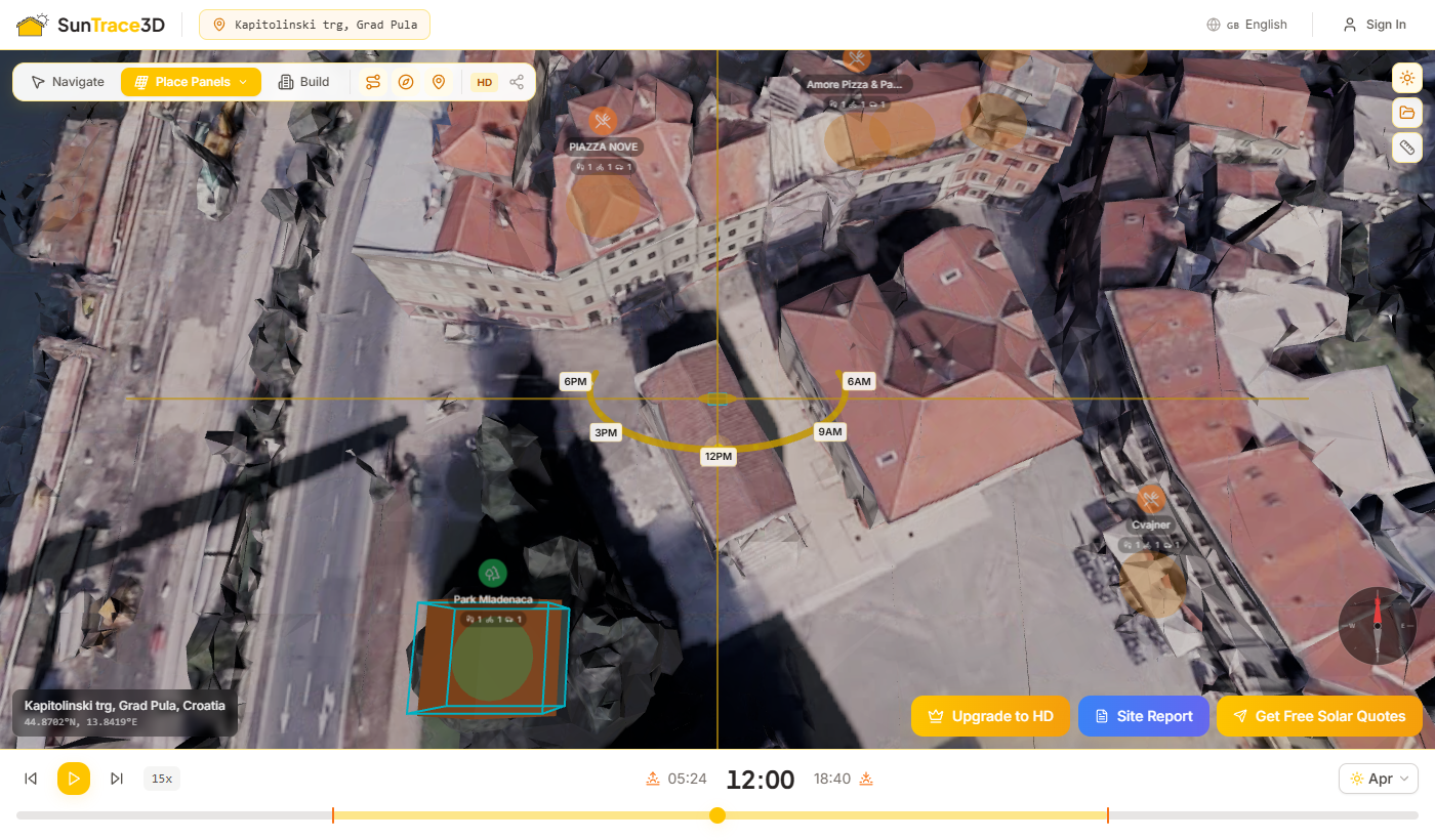
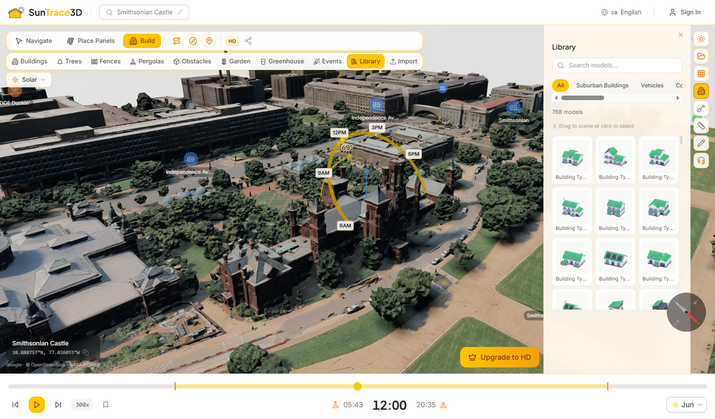
Click 'Open Viewer' from the home page. The default demo location (Pula, Croatia) loads automatically with a photorealistic 3D model.
Search a Location
Use the search bar in the header to find any address worldwide. The 3D model updates instantly when you select a new location.
Explore Shadows
Use the time slider at the bottom to see how shadows change throughout the day. Pick any date with the date picker.
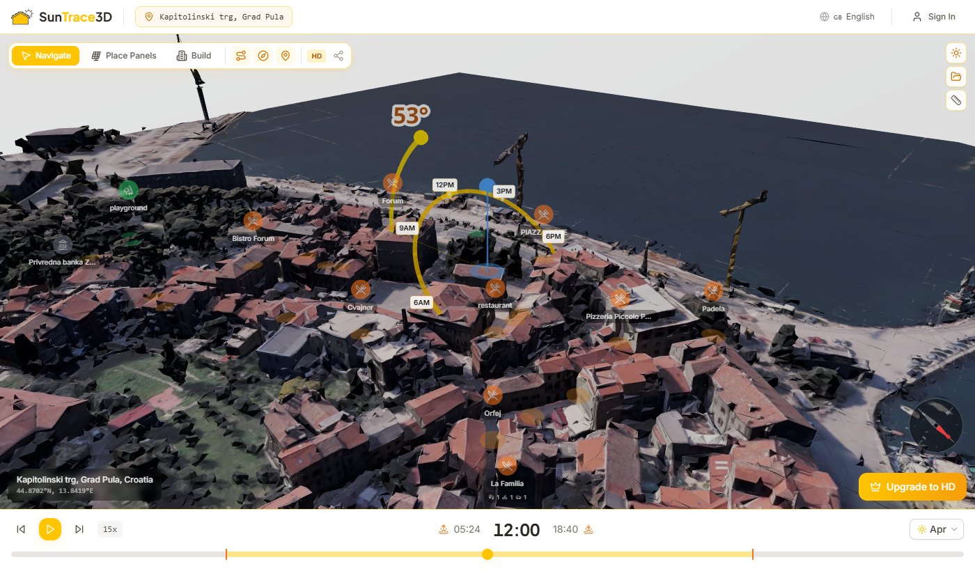
Navigate the 3D scene using your mouse or trackpad. The viewer supports orbit, pan, and zoom controls for exploring the city model from any angle.
Desktop Controls
- Left click + dragOrbit / rotate the camera around the model
- Right click + dragPan the camera (move sideways / up-down)
- Scroll wheelZoom in and out
Touch Controls
- One finger dragOrbit / rotate the camera
- Two finger dragPan the camera
- Pinch gestureZoom in and out
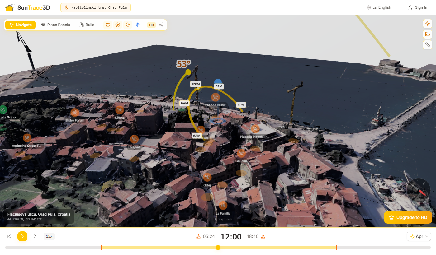
Interactive selection in Navigate mode
In Navigate mode, click any object in the scene to select it and open its configuration panel automatically. Click a solar panel to open Solar Analysis; click a building, tree, or imported model to open the Build panel. Click on empty space, or press N, to deselect everything.
The location search bar in the header lets you find any address, city, or landmark worldwide. Type an address and the system converts it to coordinates instantly.
Search tips
- 1.Type an address, city name, or landmark (e.g., "Colosseum, Rome" or "221B Baker Street, London")
- 2.Select a result from the dropdown suggestions
- 3.The 3D model loads instantly for the selected location
- 4.The URL updates with the coordinates so you can share or bookmark the location
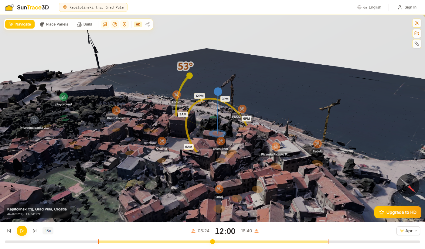
SunTrace3D calculates accurate sun positions based on your location's latitude, longitude, date, and time. Solar altitude and azimuth are computed precisely, and shadows are cast in real-time using physically-based rendering.
Time Slider
Use the horizontal slider at the bottom of the viewer to scrub through 24 hours. Watch shadows sweep across buildings as the sun moves across the sky.
Date Picker
Select any date in the header to see how shadows change with the seasons. Compare summer solstice (longest day) with winter solstice (shortest day).
Time Animation
Press the play button (or Space key) to animate the sun across the sky. Adjust the speed (15x–120x) and pick any month to compare seasonal shadow patterns. The animation loops through a full day automatically.
Understanding shadows
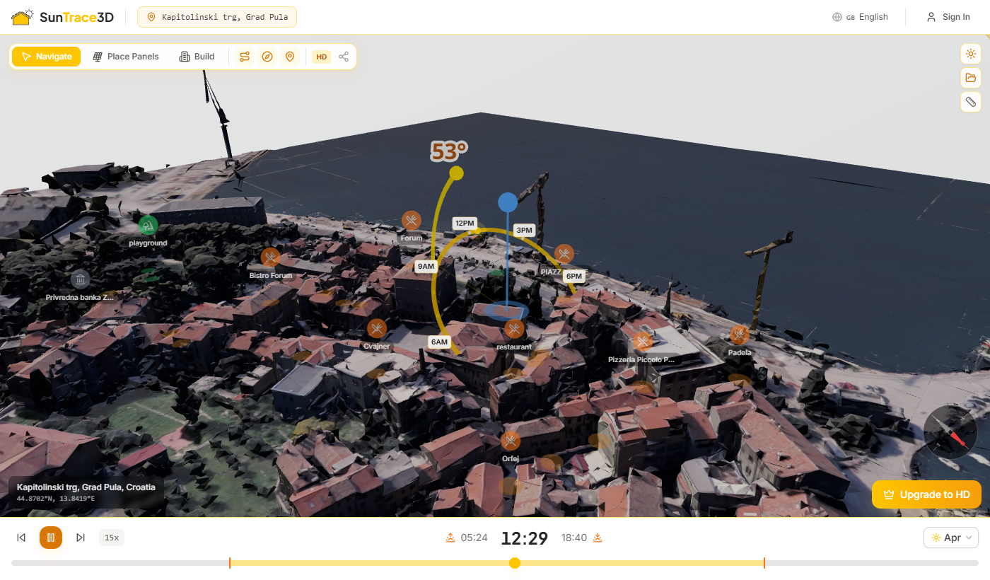
Shadow length and direction depend on the sun's altitude (height above the horizon) and azimuth (compass bearing). In the Northern Hemisphere, shadows point north at solar noon. Shadows are longest at sunrise and sunset, and shortest at solar noon. In winter, shadows are longer because the sun stays lower in the sky.
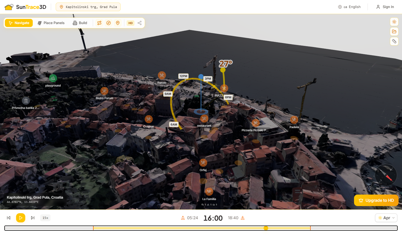
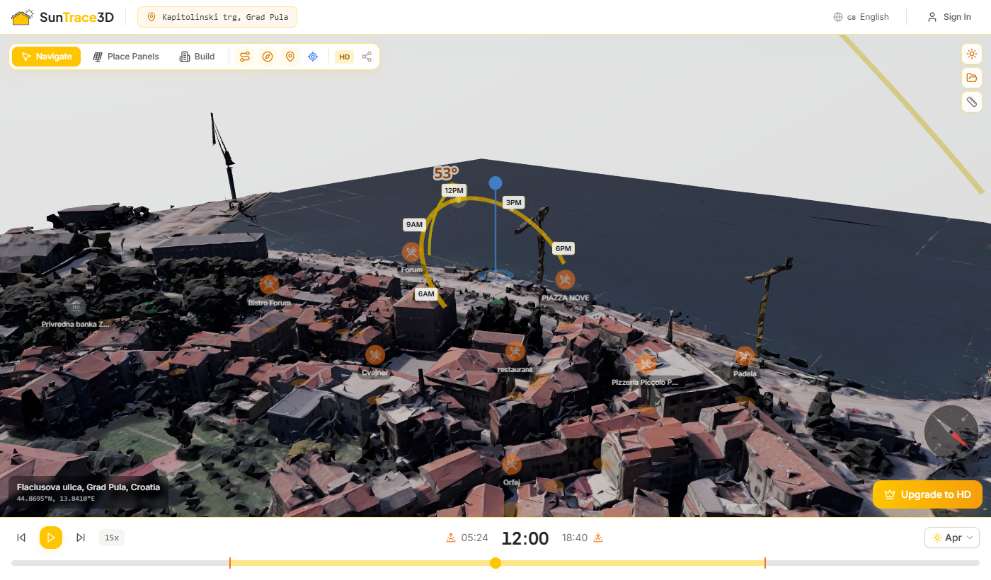
The sun path arc shows the complete trajectory of the sun across the sky for the selected date. A yellow/orange arc traces the sun's position from sunrise to sunset, with the current sun position highlighted.
What the sun path shows
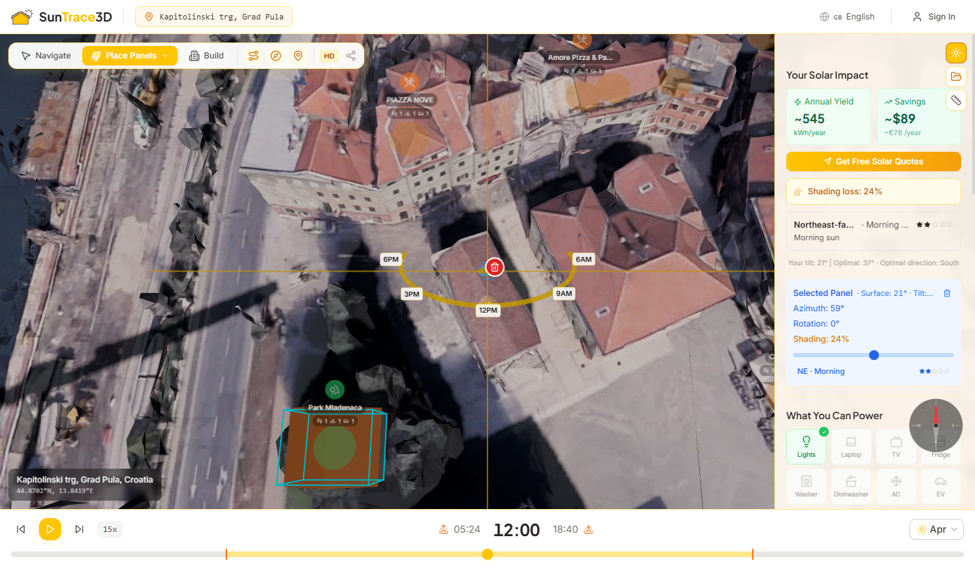
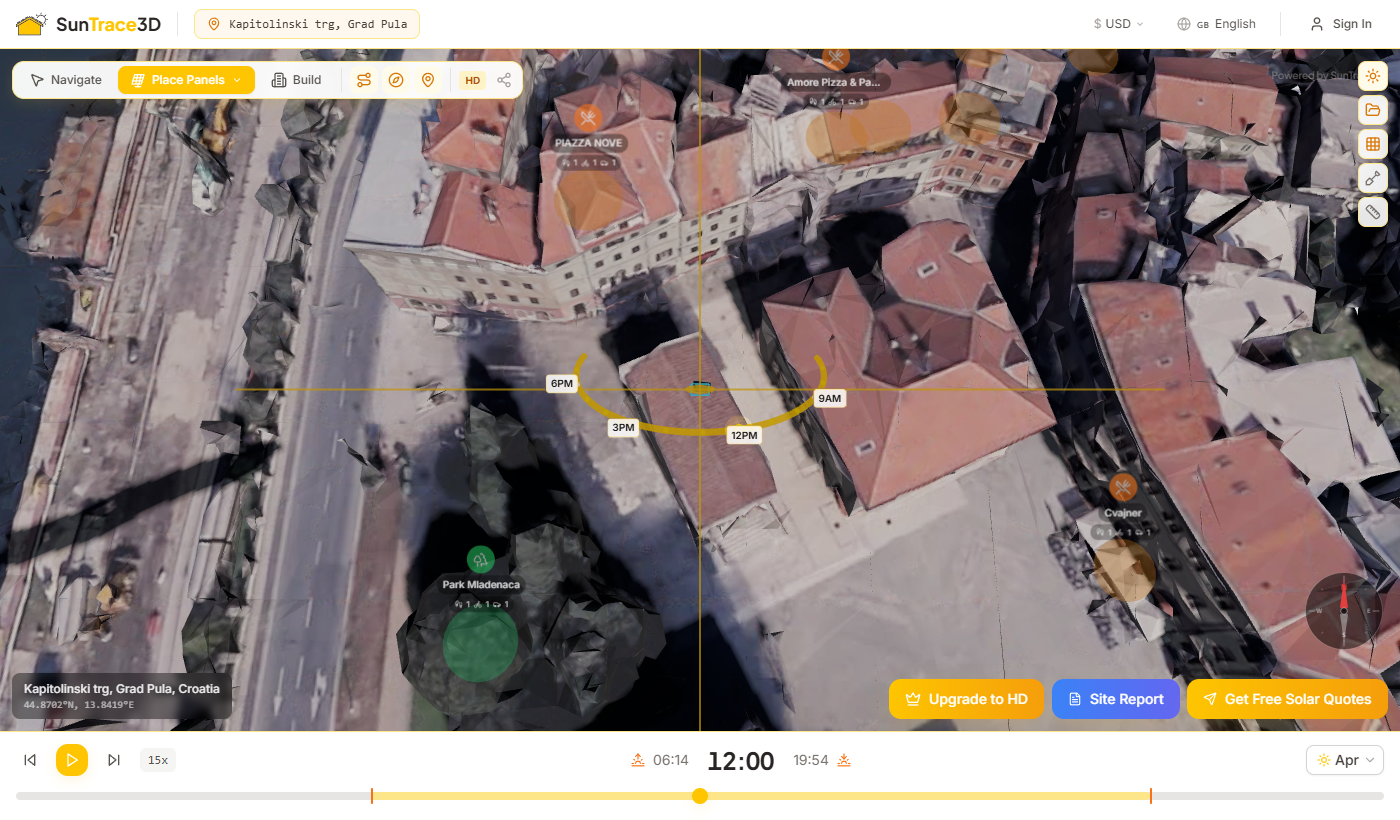
Place virtual solar panels on any rooftop in the 3D model. SunTrace3D calculates irradiance based on panel tilt, azimuth, and shading from surrounding buildings.
How to place solar panels
- 1Activate panel modeClick the solar panel button in the toolbar (bottom-left). This activates the panel placement mode.
- 2Click on a rooftopClick anywhere on a rooftop surface. A virtual solar panel appears at the clicked location.
- 3Rotate and repositionClick a placed panel to select it. Drag it to move to a new roof position. Use the rotation ring or [ ] keys to rotate the panel ±15°.
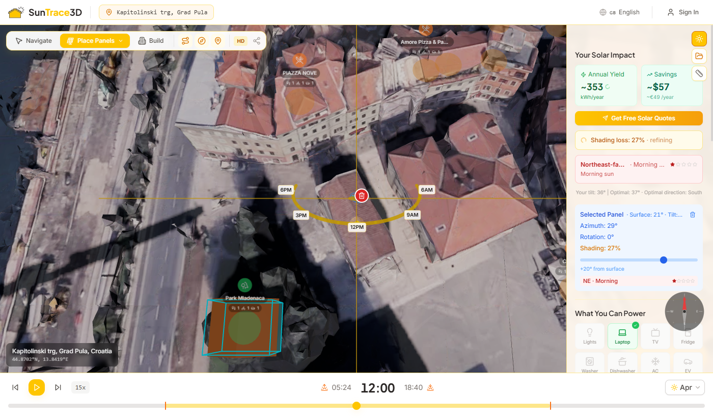
- 4Adjust tilt angleWith a panel selected, use the tilt slider in the sidebar to adjust the inclination angle (-45° to +45° from the roof surface). The panel lifts automatically to avoid clipping through the roof.
- 5Check orientation qualityThe sidebar shows the panel's surface angle, effective tilt, azimuth, and a star rating for direction quality (e.g. 'S · All-day ★★★★★' for south-facing).
- 6View energy estimatesThe solar dashboard automatically calculates annual energy yield based on your panel configuration and location. Energy updates in real-time as you adjust tilt and orientation.
Orientation Quality Rating
SunTrace3D rates each panel's orientation on a 5-star scale based on azimuth angle relative to your latitude. South-facing panels (in the northern hemisphere) receive the highest rating. The badge also shows the best sun exposure time — all-day, morning, or afternoon.
Rectangle Array Placement
For larger installations, use Rectangle placement mode to fill an entire roof area with a grid of panels in one drag — much faster than placing panels one by one.
How to place a panel array
- 1Enter Rectangle modeWhile in Place Panels mode, press R on the keyboard or select 'Rectangle' from the placement dropdown in the toolbar.
- 2Place a seed panelClick on a rooftop surface to place a single panel. This panel becomes the starting point for your grid and is automatically selected.
- 3Drag to create a gridDrag the '+' handle that appears above the selected panel. A live ghost preview shows the grid layout with cyan cells for valid positions and red cells for invalid ones.
- 4Review and releaseA floating label shows the panel count and total peak power (kWp) in real-time. Release the mouse to commit the array. All placed panels become a group that can be tilted, rotated, or deleted together.
Adjusting Panel Spacing
After placing a panel array, select any panel in the group. A 'Gap between panels' slider appears in the sidebar, allowing you to adjust spacing from 0 to 10 cm. The default gap is 2 cm.
Eraser Mode
Press E to toggle Eraser mode. Click on any placed panel to remove it individually. Press E again to return to the previous placement mode.
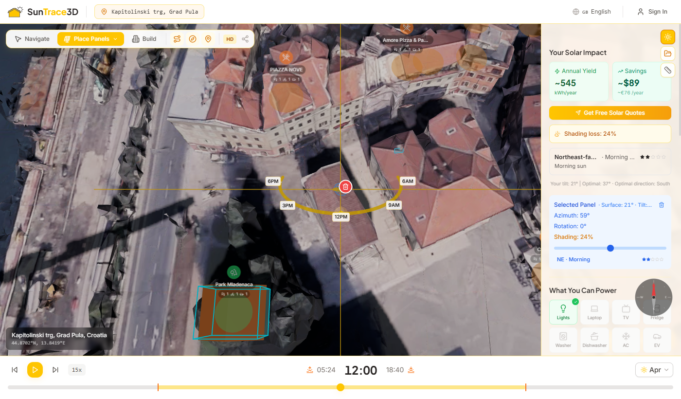
SunTrace3D automatically analyzes shading from surrounding buildings for every solar panel you place. The system simulates approximately 154 sun positions throughout the year to calculate how much each panel is blocked by nearby geometry.
How shadow analysis works
- 1Automatic detectionShadow analysis begins automatically when you place or move a panel. A spinning indicator shows while the calculation runs.
- 2Annual sun samplingThe system simulates sun positions every 15 days throughout the year, sampling every 2 hours during daylight hours — approximately 154 positions in total.
- 33D raycastingFor each sun position, a ray is cast from the panel toward the sun. If a building or other geometry blocks the ray, that time slot is counted as shaded.
- 4Weighted calculationHigher sun positions contribute more weight because the sun delivers more energy at steeper angles. Midday shading therefore impacts the result more than dawn or dusk shading.
How shading affects energy yield
The shading loss percentage is applied as a direct multiplier to the energy yield: a panel with 25% shading loss produces 25% less energy than an identical unshaded panel. Monthly estimates also reflect this — winter months may show higher losses when the sun is lower and more easily blocked by buildings.
Shading indicators
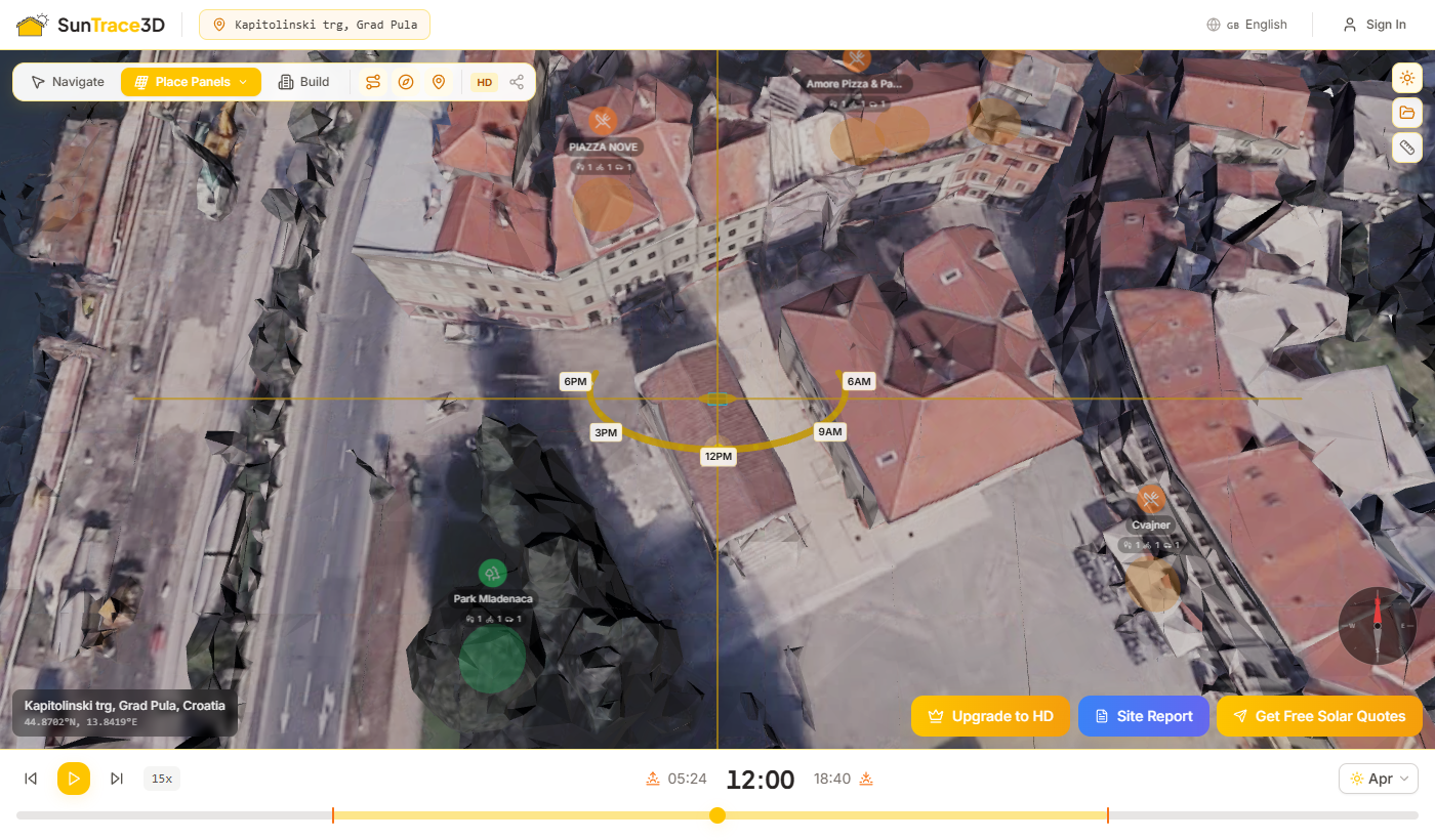
SunTrace3D estimates annual energy yield using the PVGIS (Photovoltaic Geographical Information System) database maintained by the European Commission. PVGIS provides satellite-based solar irradiance data for locations worldwide.
What's calculated
- Annual energy yield in kWh
- Peak power output in kW
- Specific yield (kWh/kWp)
- Monthly energy production breakdown
- Shading loss factor
- System losses (inverter, wiring)
Input parameters
- Panel tilt angle (0° – 90°)
- Panel azimuth (compass direction)
- Total panel area (m²)
- Panel efficiency (typically 18-22%)
- Location coordinates (automatic)
- Local solar irradiance data (PVGIS)
About PVGIS data
PVGIS uses satellite imagery and meteorological data to provide solar irradiance values averaged over many years. The data accounts for typical weather patterns, cloud cover, and atmospheric conditions. System losses of 14% are applied by default to account for inverter efficiency, wiring losses, and temperature effects.
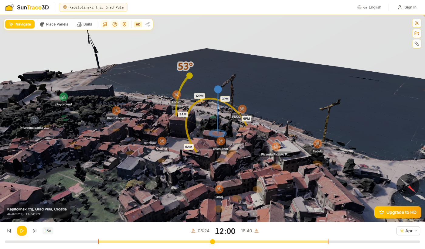
The Solar Wizard automatically detects roof surfaces and places an optimized solar panel layout with a single click. It analyzes shading across the year, avoids obstructed areas, and positions panels for maximum energy production — or to match your specific goal.
How to Use
- 1Open the WizardSwitch to Place mode, then click 'Solar Wizard' in the placement dropdown or press W. The wizard requires a paid plan (Personal or higher).
- 2Choose Your GoalSelect from four optimization strategies: Maximize Energy fills the roof, Cover My Bill matches your monthly usage, Best ROI optimizes payback period, and Go Green maximizes environmental impact.
- 3Click a Roof SurfaceClick anywhere on a roof. The wizard automatically detects the surface boundary and scans the area — you'll see golden cells appear as the detection progresses.
- 4Watch the PlacementPanels are placed one by one with a cinematic animation. The wizard selects positions with the lowest shading and groups them together for a clean, professional layout.
- 5Review & KeepReview the estimated annual yield, CO₂ offset, and bill coverage. Click 'Keep Layout' to accept or 'Start Over' to try a different roof or goal. The shading analyzer will automatically refine estimates after placement.
- 6Select EquipmentAfter panel placement, the wizard guides you through equipment selection. An inverter is automatically sized to match your array's DC capacity — for larger systems, multiple inverters are recommended with balanced string distribution. Optionally add a battery, with capacity recommended based on your energy profile and plan tier.
- 7Final System SummaryThe final results screen shows your complete system at a glance: panel count, annual energy yield, selected inverter(s), battery capacity, CO₂ offset, and estimated bill coverage percentage. Click 'Keep Layout' to commit the design or 'Start Over' to try again.
Optimization Goals
Maximize Energy
Places as many panels as possible on the detected surface for maximum annual energy generation.
Cover My Bill
Enter your monthly electricity usage in kWh, and the wizard places just enough panels to offset it.
Best ROI
Focuses on the least-shaded positions for the fastest return on investment.
Go Green
Maximizes the number of panels to achieve the highest CO₂ offset and environmental impact.
Automatic Equipment Sizing
The wizard auto-selects inverters from the CEC-certified catalog based on your panel array's total DC output. For systems exceeding a single inverter's capacity, it recommends multiple units with even string distribution. Battery recommendations are tier-gated — higher plans unlock larger storage options.
After the wizard places panels, you can still manually adjust individual panels — drag them, rotate with [ and ] keys, or delete with the eraser tool.
Ground mount arrays let you design solar installations on open terrain rather than rooftops. Draw a boundary polygon on the ground, configure tilt, azimuth, and row spacing, then instantly preview the panel layout before committing.
How to Use
- 1Select Ground Mount modeClick the Ground Mount tool (G) in the toolbar to enter drawing mode. The Ground Mount configuration panel opens in the sidebar.
- 2Draw the boundaryClick on the ground to place polygon vertices defining the array area. Close the shape by clicking near the first point — a yellow indicator appears within 3 meters.
- 3Configure array parametersAdjust tilt angle, azimuth, GCR (ground coverage ratio), panel orientation (landscape/portrait), and intra-row gap using the sidebar sliders. The row pitch updates in real time.
- 4Confirm placementReview the preview layout showing valid (cyan) and invalid (red) panel positions within your boundary. Click Confirm to place the array.
- 5Manage arraysView array details in the sidebar including panel count, peak power, tilt, azimuth, GCR, and row pitch. Use the Redraw button to reshape an array with preserved settings, or delete it entirely.
Ground mount arrays require a Pro plan or higher. Pro allows up to 2 arrays with 20 panels total. Business and Enterprise plans include unlimited ground mount arrays.
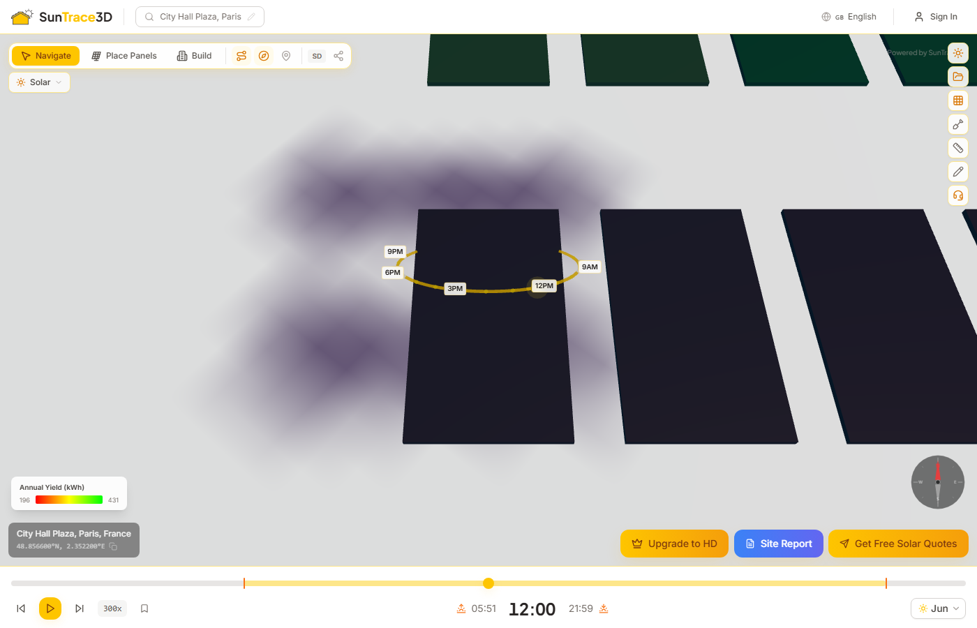
Visualize energy performance across your entire panel array with a color-coded heatmap. Each panel is shaded from red (low annual yield) through yellow (mid-range) to green (high yield), making it easy to spot underperforming panels at a glance.
How to use the panel heatmap
- 1Place solar panelsPlace one or more solar panels on the 3D model and wait for the energy calculation to complete. The annual yield per panel must be computed before the heatmap can be displayed.
- 2Open the heatmap toggleIn the Solar sidebar, click the 'Panel Heatmap' button. It appears below the Smart Suggestions section once panels are placed and energy has been calculated.
- 3Read the gradient legendA color legend appears in the bottom-left corner of the viewer showing the min and max annual kWh values. Red panels produce the least energy; green panels produce the most.
- 4Toggle offClick the heatmap button again to return panels to their default color scheme.
Shadow-Aware Analysis
The heatmap reflects real shading conditions. Panels blocked by nearby buildings, trees, or imported 3D models will show lower yield and warmer colors.
Color Gradient
Red indicates the lowest annual yield in the array. Yellow marks mid-range performance. Green marks the highest-performing panels. The gradient automatically scales to your array's min/max values.
Use the heatmap to compare panels with different orientations or shading conditions. Panels facing away from the sun or in heavy shadow will appear red, helping you optimize your layout.
SunTrace3D offers two quality levels for 3D models. The quality badge in the viewer toolbar shows the current mode.
Standard Detail
Available for select demo locations on the free tier. Pro and Business subscribers can generate SD and HD models at any address. Models load instantly with moderate geometric and texture detail. Perfect for quick shadow studies and solar analysis.
Demo locations — no account needed to try
High Definition
Available on the Pro tier. Photorealistic models with maximum texture and geometric detail. Individual building features, vegetation, and street-level detail are clearly visible.
Pro subscription — €9/month
The compass overlay in the viewer shows true north orientation relative to your current camera angle. This is essential for understanding shadow directions and optimal solar panel orientation.
Reading the compass
- The compass rotates as you orbit the 3D model, always pointing toward true north
- In the Northern Hemisphere, south-facing panels receive the most sunlight
- Use the compass to verify panel azimuth when placing solar panels
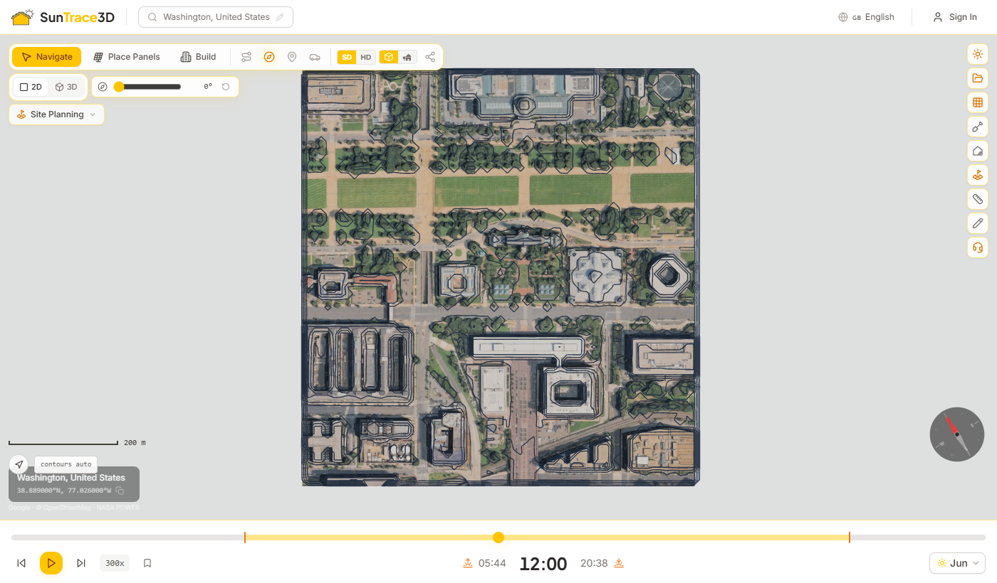
Plan mode turns the viewer into a true top-down drawing. It uses an orthographic camera, so there is no perspective: building sides disappear, distances read the same everywhere on screen, and a site plan can be measured rather than just looked at.
Using plan mode
- 1Switch to 2DClick 2D in the view toggle at the top left, or press 2. Press 3 or click 3D to return; your 3D viewpoint is restored exactly where you left it.
- 2Read the drawingA scale bar in the corner resizes as you zoom. Pan by dragging and zoom with the mouse wheel; the view stays locked flat.
- 3Rotate to project northDrag the project north slider to align the drawing with your site. It rotates the view only — coordinates, measurements and exports are never changed.
- 4Show or hide contoursContour lines are generated from the loaded terrain at an automatic interval. Use the contours button to turn them off or back on.
Framed around your panels
When a side panel is open, the plan is fitted to the part of the screen you can actually see, so nothing is hidden behind it.
Contours from the real model
Contours are sampled from the 3D model you have loaded, not from a separate elevation source, so they follow the same ground your design stands on.
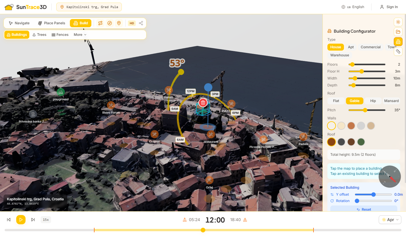
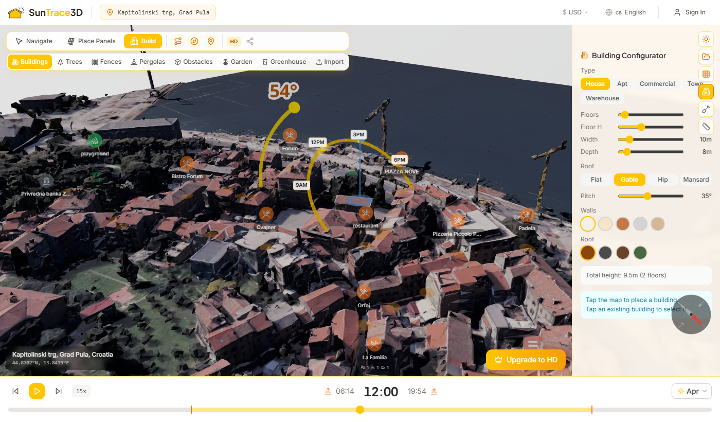
Build mode lets you place procedural buildings into the 3D scene. These buildings cast and receive shadows just like real-world models, making it easy to study how a proposed development would affect sunlight on surrounding properties.
How to place buildings
- 1Activate Build modeClick the Build button in the toolbar or press B. The sidebar opens automatically with the Building Configurator.
- 2Choose a building typeSelect from five types: House, Apartment, Commercial, Townhouse, or Warehouse. Each type loads sensible default dimensions and roof style.
- 3Adjust dimensions and styleFine-tune floors (1–20), floor height (2.5–4m), width (4–50m), and depth (4–50m). Choose a roof type and pick wall and roof colors from the swatch palettes.
- 4Click the ground to placeClick anywhere on the ground in the 3D scene. The building appears at the clicked location using your current configurator settings.
- 5Select and adjustClick a placed building to select it. When selected you can rotate it, adjust the vertical offset, apply new settings, or delete it using the sidebar controls.
Building Types
House
2 floors, 10 × 8 m, gable roof at 35°. Compact residential building.
Apartment
5 floors, 20 × 12 m, flat roof. Multi-story residential block.
Commercial
3 floors, 25 × 15 m, flat roof. Office or retail building.
Townhouse
3 floors, 6 × 12 m, gable roof at 40°. Narrow and deep.
Warehouse
1 floor, 30 × 20 m, flat roof. Wide, low industrial building.
Roof Types
Shadow analysis with buildings
Placed buildings participate fully in the shadow simulation. Scrub the time slider to see how a proposed building would cast shadows on neighbouring rooftops, gardens, or solar panels throughout the day and across seasons.
Build mode includes a Scene Objects panel for adding trees, fences, pergolas, and obstacles (chimneys, poles, cylinders) to the 3D scene. These objects cast and receive shadows, letting you study how landscaping and rooftop features affect solar panel performance.
How to place scene objects
- 1Enter Build modeClick the Build button in the toolbar or press B. The sidebar shows category tabs at the top: Buildings, Trees, Fences, Pergolas, and Obstacles.
- 2Choose a category and styleClick a category tab, then select a shape or style. Trees offer round, oval, conifer, palm, and columnar shapes. Fences include wood, brick, concrete, and hedge. Pergolas come in flat, louvered, and awning styles. Obstacles include box, cylinder, chimney, and pole shapes.
- 3Adjust dimensions and colorUse the sliders to set height, width, depth, or canopy diameter. Pick a color from the swatch palette. Trees can be set as deciduous (seasonal leaf loss) or evergreen.
- 4Click to placeClick on the ground or on a building surface to place the object. Once placed, click to select it, then drag to reposition, use [ ] to rotate, or press Delete to remove.
Object Categories
Trees
Deciduous and evergreen trees with configurable height, canopy size, and trunk height. Five shapes: round, oval, conifer, palm, columnar.
Obstacles
Rooftop obstacles like chimneys, vents, and poles. Four shapes: box, cylinder, chimney, pole. Place on buildings to study shading impact.
Fences
Perimeter fences and walls with adjustable length, height, and thickness. Styles: wood, brick, concrete, hedge.
Pergolas
Shade structures with width, depth, and tilt controls. Three styles: flat, louvered, and awning.
Shadow interaction
All scene objects participate in the shadow simulation. Trees and fences cast realistic shadows that affect solar panels — the shadow analysis automatically accounts for these obstructions when calculating shading loss.
Building attachment
Objects placed on a building surface automatically attach to that building. When you rotate or move the building, attached objects move with it. Drag an object off the building to detach it.
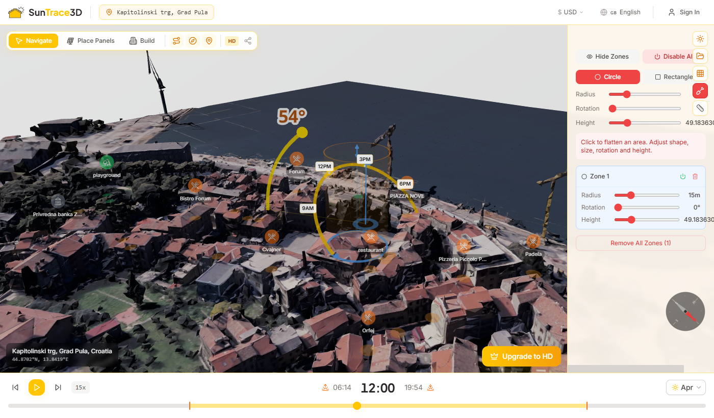
The Bulldozer tool lets you flatten terrain in the 3D scene by defining clearing zones. 3D models often include trees, bushes, and uneven ground — use the Bulldozer to remove these before placing solar panels or buildings for accurate shadow analysis.
How to use the Bulldozer
- 1Activate the BulldozerClick the Shovel icon in the left sidebar toolbar. The button turns red when bulldozing mode is active.
- 2Choose a zone shapeSelect Circle or Rectangle in the configurator. Set the dimensions — radius for circles, or width, depth, and rotation for rectangles. Adjust the height to control how much terrain is flattened.
- 3Click to place a clearing zoneClick anywhere on the ground in the 3D scene. A semi-transparent zone appears showing the area that will be cleared.
- 4Manage zonesClick a placed zone to select it and adjust its size or shape. Toggle individual zones on/off with the power button, or use the global Show/Hide and Enable/Disable All controls.
Circle Zone
A circular clearing area defined by radius (5–50 m). Best for clearing individual trees or small obstructed areas.
Rectangle Zone
A rectangular clearing area with configurable width (5–80 m), depth (5–80 m), and rotation. Ideal for preparing building sites or large panel array areas.
When to use the Bulldozer
3D models often include vegetation and terrain features that interfere with shadow analysis and panel placement. Use the Bulldozer to clear these areas and create a clean surface for accurate solar studies.
Tip
Bulldozer zones are included in energy yield calculations. When you clear terrain beneath or near solar panels, the energy estimate automatically accounts for the changed shading environment.
Draw custom building footprints directly on the terrain by clicking to create a polygon outline. SunTrace3D automatically converts your polygon into one or more 3D buildings that you can place solar panels on, analyze for shadows, and include in energy calculations.
How to draw a building
- 1Activate Draw a HouseClick the house icon in the sidebar toolbar or press H. An animated tutorial shows how the tool works.
- 2Click to place pointsClick on the terrain to place corner points of your building footprint. You need at least 3 points.
- 3Close the polygonClick near the first point, double-click, or press Enter to close the shape. The camera automatically transitions to show a 3D preview of your buildings.
- 4Configure and confirmAdjust floors (1–20), floor height, roof type (flat or pitched), roof pitch (15–60°), wall color, and roof color. Click Place Buildings to add them to your scene.
Building Configuration
Set the number of stories, floor height, roof style, pitch angle, and colors. Complex polygons are decomposed into multiple rectangular buildings to fit the outline. The total footprint area and building count are shown in the panel.
No Buildings Detected
If you load a location where no buildings are detected near the center, a helpful prompt appears suggesting you draw your own building. Click the button to jump straight into drawing mode.
Tip
The total footprint area and number of generated buildings are shown in the configuration panel. Complex polygons may be decomposed into multiple rectangular buildings to fit the outline.

The Sunlight Heatmap displays a color-coded ground grid showing how many hours of direct sunlight each area receives. Use it to identify the sunniest and shadiest spots on your property — perfect for planning solar panel placement or garden beds.
How to use the heatmap
- 1Open the Heatmap panelClick the grid icon in the left sidebar to open the Sunlight Heatmap panel. Set the width and depth of the analysis area (10–20 m free, up to 100 m for Pro).
- 2Show the heatmapClick 'Show Heatmap'. The system computes sunlight hours for every grid cell and renders the color-coded overlay on the ground.
- 3Adjust month and opacitySelect a specific month or 'Year' for the annual average. Adjust opacity and rotation to fine-tune the visualization. The heatmap recalculates when you change the month.
Color scale
Larger heatmaps on paid plans
Free accounts can create heatmaps up to 20 × 20 meters. Personal subscribers can extend the heatmap to 100 × 100 meters. Business subscribers can analyze areas up to 1000 × 1000 meters for large commercial sites, solar farms, or agricultural land.
The Garden Planner helps you design garden beds using a database of 50+ plants, each with documented sunlight requirements. Combined with the Sunlight Heatmap, it automatically checks whether your chosen plants will thrive in the available light conditions.
How to plan a garden
- 1Enable the heatmapTurn on the Sunlight Heatmap first (see previous section) so the system has sunlight data for your property.
- 2Open the Garden panelClick the flower icon in the sidebar to open the Garden Planner panel. Browse the plant catalog organized by category: vegetables, herbs, fruits, flowers, and shrubs.
- 3Select a plant and bed shapeClick a plant to select it. Choose a bed shape — rectangle, circle, or L-shape — and adjust the width, depth, and raised bed height using the sliders.
- 4Place and check compatibilityClick on the ground to place the garden bed. The system cross-references the bed's location with heatmap data and shows a compatibility indicator: ideal (green), acceptable (yellow), or not suitable (red).
Plant Categories
Vegetables
Tomatoes, peppers, lettuce, carrots, and more — with sun and harvest time data
Herbs
Basil, rosemary, thyme, mint, and more — each with ideal sun zone
Fruits
Strawberries, blueberries, and orchard fruits with season data
Flowers
Sunflowers, lavender, roses, and more for ornamental beds
Shrubs
Hedges and bushes with shade tolerance info
Automatic compatibility checking
The Climate Data panel appears in the Solar Analysis sidebar whenever you have solar panels placed. It shows location-specific climate metrics that directly affect solar panel performance — cloud cover losses, ambient temperature, and heat-related efficiency losses.
Cloud Loss
The percentage of solar energy lost to cloud cover at your location, derived from satellite-measured clear-sky index data. Higher values mean more clouds and less available sunlight.
Average Temperature
The annual average air temperature at your location in °C. This baseline is used to estimate panel cell temperature and thermal efficiency losses.
Heat Loss
Estimated efficiency loss due to high panel temperatures. Solar panels lose approximately 0.29% efficiency for each degree above 25°C cell temperature.
Monthly Cloudiness
A sparkline chart showing the clear-sky index for each month (January to December). Green bars indicate clear months with high solar yield; blue bars indicate cloudy months.
Data source
Climate data comes from NASA POWER (CERES SYN1deg + MERRA-2), providing a 22-year global climatology. The data automatically adjusts energy yield estimates for realistic local weather conditions.
When you place solar panels, SunTrace3D automatically estimates the installation cost, annual electricity savings, and payback period based on regional pricing data.
Cost Breakdown
The Installation Cost section in the sidebar shows a detailed breakdown including panel cost, installation labor, and inverter/balance-of-system costs. Prices are adjusted to your region and displayed in your selected currency.
Annual Savings & Payback
Based on the estimated annual energy yield and local electricity prices, SunTrace3D calculates your annual savings and the number of years until the system pays for itself.
Government Incentives
Where available, the calculator shows estimated government subsidies, tax credits, or feed-in tariffs that reduce your effective cost and shorten the payback period.
Request a Quote
Scroll to the foot of the Solar sidebar and click 'Get Free Solar Quotes' to submit your solar analysis to local installers. The form pre-fills with your system specs, location, and estimated costs for a personalized proposal.
The Solar Impact section visualizes the environmental benefits of your solar panel system. It appears in the sidebar whenever you have panels placed in the scene.
CO₂ Offset
See how many kilograms of CO₂ your system would avoid annually. This is calculated from your estimated energy yield and regional grid emission factors.
Appliances Powered
A visual grid of 9 common household items shows which appliances your system can power — from light bulbs and laptops to refrigerators, air conditioning, and electric vehicles. Powered items light up in green.
Shading & Orientation Ratings
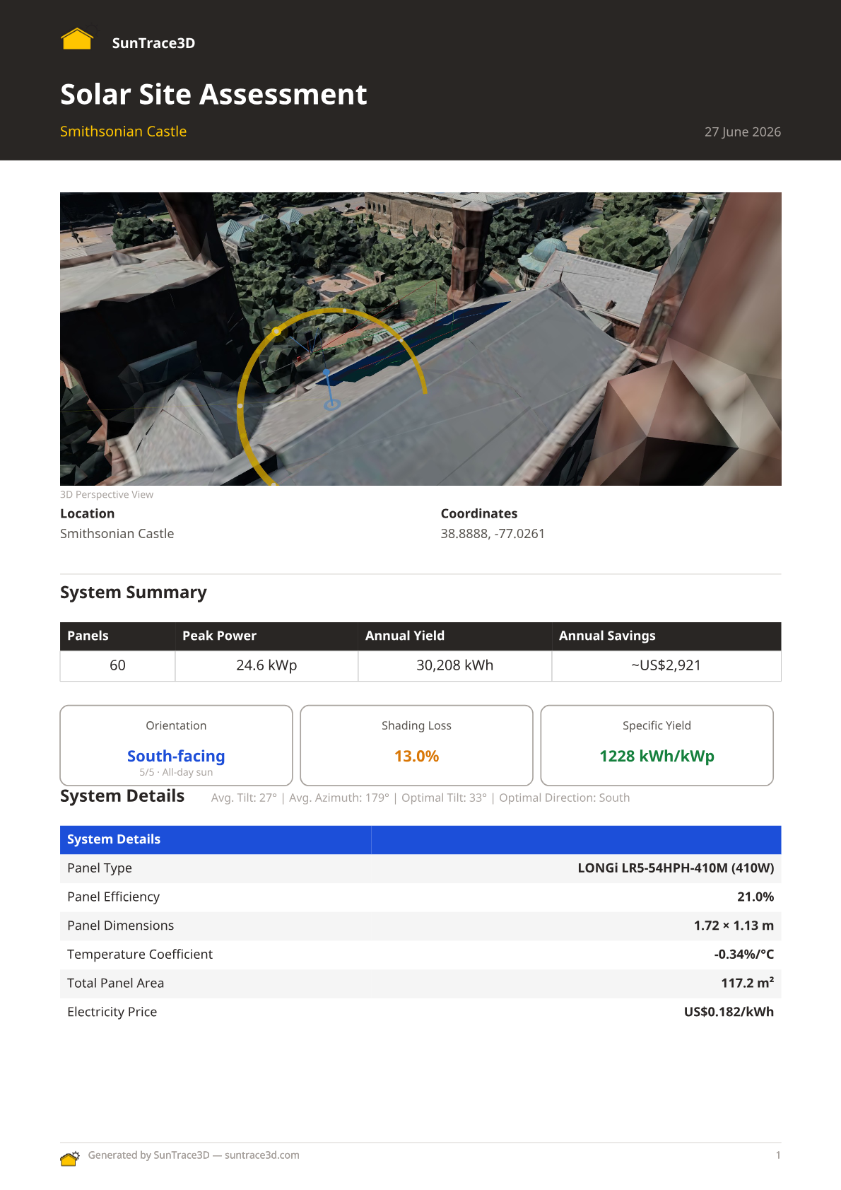
Generate a professional PDF site report summarizing your entire solar analysis. The report includes 3D views, system specifications, energy yield estimates, engineering details, financial analysis, and environmental impact — ready to share with clients or installers.
How to generate a site report
- 1Place solar panelsSet up your solar panel installation in the 3D viewer. The report button appears once you have panels placed with energy yield results.
- 2Click 'Site Report'Click the blue Site Report button at the bottom of the viewer. Sign in if prompted — a free account is required.
- 3Fill in detailsOptionally enter your company name, client name, upload a company logo, and add notes. You can also adjust the total investment amount.
- 4Generate and downloadClick 'Generate PDF Report'. The system captures 3D views of your scene, builds the report, and offers a PDF download.
What's in the report
- 3D perspective and top-down views of the solar installation
- System summary: panel count, peak power, annual yield, orientation, shading loss
- Detailed system specs: panel type, efficiency, dimensions, tilt, azimuth
- Monthly energy production chart
- Financial analysis: cost breakdown, payback period, government incentives
- Household appliances the system can power
- Custom branding with company logo and installer details
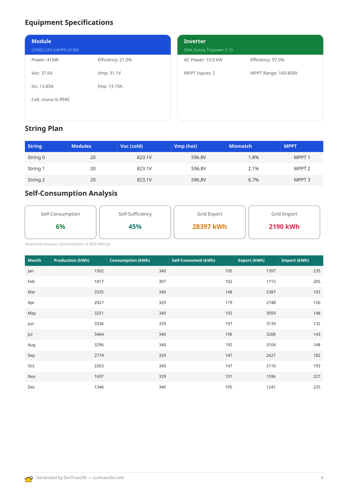
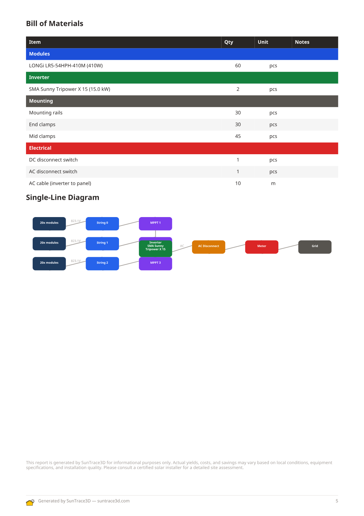
- String plan table with voltage limits, MPPT assignment, and multi-inverter support
- Auto-generated single-line diagram (SLD) showing PV strings, inverters, and grid connection
- Cable sizing recommendations with voltage drop calculations per string
- Self-consumption and self-sufficiency analysis with hourly load matching
- Battery storage simulation results and dispatch analysis
- Bill of materials with module, inverter, mounting, and cable quantities
- Loss waterfall chart showing energy losses from gross to net production
Engineering sections (string plan, SLD, cable sizing, self-consumption, battery, BOM) appear automatically when you have selected a module and inverter from the engineering catalog.
Custom branding
Upload your company logo and enter your company name to create branded reports. The logo appears in the report header alongside the SunTrace3D branding — perfect for solar installers sending proposals to clients.
The Loss Waterfall Chart in the PDF site report provides a detailed visual breakdown of energy losses from gross solar potential to net delivered energy. Each loss category is shown as a colored bar segment, making it easy to identify the largest efficiency drains in your system.
How to view the loss waterfall
- 1Place panels and calculate energyPlace solar panels on the 3D model and wait for the energy calculation to complete. The loss waterfall uses both measured site-specific losses and standard industry values.
- 2Generate the PDF site reportClick the 'Site Report' button in the Solar sidebar to generate a PDF report. The loss waterfall chart is included automatically in the report.
- 3Review loss categoriesThe chart shows gross energy on the left and net energy on the right, with each loss category displayed as a labeled bar segment in between. Hover-friendly labels show both percentage and absolute kWh loss for each category.
Measured Losses
Shading, cloud cover (Kc factor), temperature degradation, panel mismatch, and cable losses are computed from your actual site data and panel configuration.
Industry Defaults
Inverter efficiency, DC/AC wiring losses, soiling, light-induced degradation (LID), and system availability use standard industry reference values when site-specific measurements are not available.
The waterfall replaces the old flat 14% system loss estimate with a transparent, itemized breakdown. Measured losses are site-specific; industry defaults use conservative reference values.
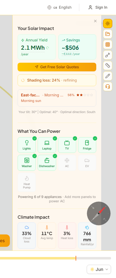
Generate professional PDF quotes to send to prospective clients. Each quote includes system specifications, investment breakdown, projected savings, payback period, warranty terms, and applicable financial incentives — all populated automatically from your solar analysis.
How to generate a quote
- 1Complete your solar designPlace solar panels on the 3D model and wait for the energy calculation to complete. The quote pulls data from your panel layout, selected equipment, and energy yield results.
- 2Open the report modalClick the report button in the Solar sidebar to open the report generation dialog. You will see options for both site reports and client quotes.
- 3Configure quote settingsEnter client details, adjust system pricing, electricity rates, and any applicable incentives or rebates. The quote preview updates in real time as you change parameters.
- 4Download the PDFClick Generate to create a branded PDF document. The quote includes a cover page, system overview, financial analysis with payback chart, warranty terms, and next steps — ready to email or print for your client.
Financial Projections
The quote calculates total investment, annual savings, cumulative savings over the system lifetime, and payback period. It also factors in local electricity price escalation and panel degradation rates.
Professional Formatting
Quotes are generated as multi-page A4 PDF documents with consistent branding, clear section headings, and a professional layout suitable for client presentations.
Quotes use the same solar analysis data as site reports but present it in a client-facing format focused on investment return rather than technical specifications. You can generate both a technical site report and a client quote from the same design.
Speed up your workflow with keyboard shortcuts. These work whenever the viewer is focused and no text input field is active.
General
- Ctrl+ZUndo last action
- Ctrl+YRedo last undone action
- Shift+ClickAdd / remove from multi-selection
- Ctrl+CCopy selected items
- Ctrl+VPaste copied items
Mode & Time
- NSwitch to Navigate mode
- PSwitch to Place Panels mode
- BSwitch to Build mode
- MMeasure distances
- DDraw annotations
- SpacePlay / pause time animation
- ← →Skip time back / forward 15 min
Build Mode (selected building)
- [ ]Rotate selected building ±15°
- DeleteRemove selected building
- ↑ ↓Raise / lower building ±0.5 m
Panel Mode (selected panel)
- [ ]Rotate selected panel ±15°
- DeleteRemove selected panel
- RToggle Rectangle placement mode
- EToggle Eraser mode
Tip
On mobile and touch devices, all building controls (rotation, vertical offset, delete) are available as sliders and buttons in the sidebar when a building is selected.
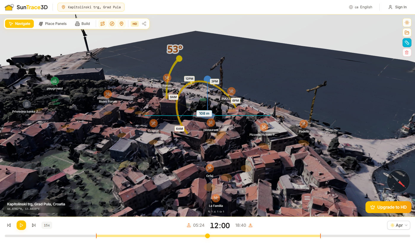
Measure real-world distances directly in the 3D scene. The measurement tool calculates the straight-line distance between any two points you click.
How to measure distances
- 1Activate measurement modeClick the ruler button in the sidebar toolbar (or press M). Your cursor changes to a crosshair.
- 2Place the first pointClick anywhere on the 3D scene to set the starting point. A cyan marker appears.
- 3Place the second pointClick a second location. A line connects the two points with the distance displayed in meters.
- 4Add more measurementsKeep clicking to add additional measurements. Click on any measurement to select it, then press Delete to remove it.
Measurement tips
- Measurements work on terrain, buildings, and rooftops
- Press Escape to cancel a pending measurement point
- Use the Clear button to remove all measurements at once
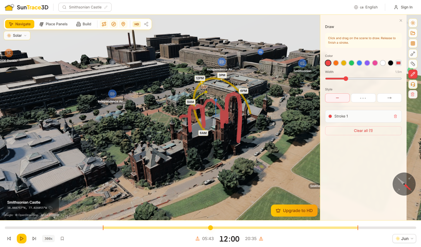
Annotate your 3D scene with freehand drawings that follow the terrain and building surfaces. Use colored strokes to mark areas of interest, add text labels, and measure enclosed areas. Drawings are saved with your project.
How to use the draw tool
- 1Activate draw modeClick the pencil button in the sidebar toolbar (or press D). Your cursor changes to a crosshair and the Draw panel opens.
- 2Draw a strokeClick and drag on the 3D scene to create a freehand stroke. The stroke follows the terrain and building geometry. Release the mouse button to finalize.
- 3Close a loop for area measurementDraw back to the starting point to close the loop. The enclosed area is automatically calculated and displayed in square meters with a semi-transparent fill.
- 4Customize and manage strokesChange stroke color, width, and style (solid, dashed, arrow) in the Draw panel. Click a stroke to select it and add a text label. Press Delete to remove selected strokes.
Drawing tips
- Strokes follow terrain, buildings, and rooftops — they snap to scene geometry automatically
- Close a loop by drawing back to the start point to see the enclosed area in m²
- Press Escape to cancel a stroke in progress or exit draw mode
Toggle Points of Interest (POI) to discover nearby amenities and landmarks overlaid on the 3D map. POI markers show restaurants, schools, shops, healthcare, and other categories.
How to use Points of Interest
- 1Toggle POI onClick the map pin button in the toolbar to enable POI markers. Nearby locations load automatically based on your current map center.
- 2Browse markersMarkers appear at real-world positions in the 3D scene. Zoom in to see names and details; zoom out and they simplify to compact icons.
- 3Click to highlightClick any POI marker to highlight it and see more details. Click again to deselect.
Available categories
Education, Healthcare, Shopping, Transport, Recreation, Dining, and Services — covering schools, hospitals, supermarkets, bus stops, parks, restaurants, and more.
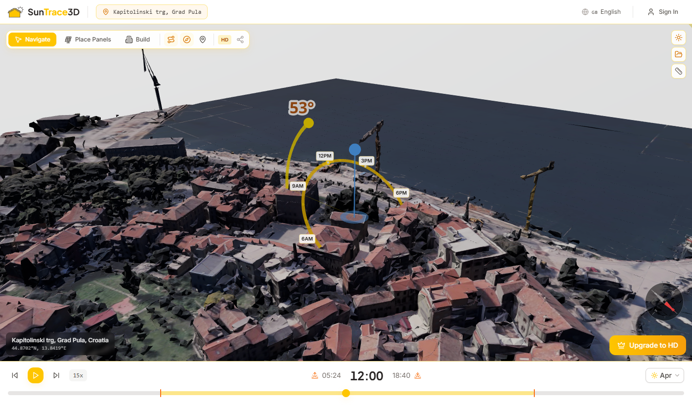
SunTrace3D offers two types of 3D models. The model type toggle in the viewer toolbar lets you switch between them. Switching regenerates the model for your current location.
Standard 3D Model
Block-style buildings with flat roofs extruded from footprint data. Loads quickly and provides accurate building placement and shadows for solar analysis.
Realistic 3D Model
Detailed building geometry with accurate roof pitches, chimneys, and textured facades. Provides the most lifelike representation of your site.
Automatic fallback
If the realistic model is unavailable for your location, the standard model is shown automatically. A small indicator appears next to the toggle when this happens.
The 3D scene includes animated vehicles and pedestrians that move along real roads, bringing the environment to life. Low-poly cars, buses, and pedestrians travel along actual road networks, making it easier to judge scale and get a realistic sense of the surroundings.
Automatic
Ambient life loads automatically when the scene and road data are ready. No setup or configuration is required.
Real road networks
Vehicles follow actual road paths from the map data, not random paths. This provides an authentic sense of movement and activity.
Scale reference
The animated figures provide an intuitive sense of scale when assessing building heights, panel sizes, and shadow lengths.
Tip
Ambient life is automatically hidden during screenshot captures and video recordings to keep outputs clean and deterministic.

SunTrace3D works without an account for basic shadow simulation and solar analysis. Create a free account to save your work, upgrade to Pro for HD models and unlimited tools, or choose Business for unlimited everything and commercial use.
Account features
Free account
- 3D city model viewer
- Full shadow simulation
- Up to 8 solar panels
- Up to 5 scene objects
- Up to 3 custom buildings
Pro (€9/mo)
- HD photorealistic models
- Unlimited panels, objects & buildings
- Save projects & import 3D models
- Compliance reports & photo export
- No watermark on reports
Business (€99/mo)
- Unlimited panels, ground mounts & heatmaps
- Real estate scoring & PDF reports
- Embeddable viewer & lead capture
- API access (500 models/mo)
- Export the full 3D scene as GLB/OBJ
Enterprise (custom)
- White-label branding
- Custom CRM integrations
- Dedicated support & SLA
- Custom API volume
Managing your subscription
Click the user menu in the viewer header to access your account settings and subscription portal. You can upgrade, downgrade, or cancel at any time.
Save your complete analysis setup — including location, solar panels, buildings, quality mode, and date/time — as a named project. Load it later to pick up exactly where you left off.
How to save and load projects
- 1Sign inCreate an account or sign in. Projects are stored server-side and tied to your account.
- 2Open the sidebarClick the sun icon in the top-right corner of the viewer. Scroll down to the Projects section at the bottom of the sidebar.
- 3Save current sceneClick "Save current scene", enter a project name, and press Save. The entire scene state is captured.
- 4Load a projectClick a saved project in the list to restore it. Location, model, panels, buildings, and time settings are all restored automatically.
What's saved in a project
- Location (latitude, longitude, and name)
- Quality mode (SD or HD)
- All solar panels with tilt, azimuth, and position
- All placed buildings with type, dimensions, position, and rotation
- All scene objects (trees, fences, pergolas, obstacles)
- Selected date and time of day
- Imported 3D models (position, rotation, and scale preserved)
Unsaved Changes Protection
When you try to load a different project while you have unsaved changes, a confirmation dialog appears warning you that your work will be lost. You can choose to discard and load the new project, or cancel and save your current work first.
Import custom 3D models into your scene to accurately represent existing structures, machinery, or any object that affects shading on your solar panels.
How to import a 3D model
- 1Switch to Build modePress B or click the Build button in the toolbar to enter Build mode.
- 2Open the Import tabClick the Import tab (upload icon) in the Build panel sidebar.
- 3Upload your GLB fileDrag and drop a .glb file onto the upload area, or click to browse. Maximum file size is 50 MB.
- 4Position the modelThe model appears at the scene origin. Use the Move, Rotate, and Scale buttons in the panel to switch gizmo modes, then drag the handles in the 3D view to position it precisely.
- 5Fine-tune with numbersEnter exact values in the Position (m), Rotation (°), and Scale fields for precise placement.
File requirements
Only .glb (binary glTF) files are supported. Maximum 50 MB per file. Models are stored securely in the cloud and load automatically when you reopen a saved project.
Transform gizmos
- Move — drag the coloured arrows to reposition along X, Y, or Z axis
- Rotate — drag the rings to spin the model around each axis
- Scale — drag the handles to resize uniformly or per-axis
3D model import is a Pro feature. Upgrade to Pro to unlock custom model placement.
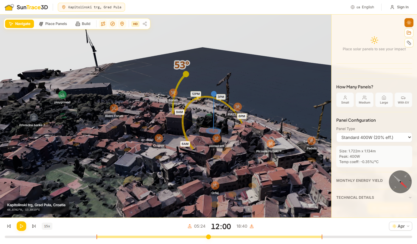
The Model Library provides over 750 ready-to-use 3D models organized into seven categories — suburban buildings, vehicles, commercial buildings, characters, nature, building parts, and trains. Browse, search, and place models directly into your scene for realistic shadow analysis and urban planning.
How to use the Model Library
- 1Open the LibraryEnter Build mode by clicking the Build button or pressing B. Select the Library tab at the top of the sidebar panel.
- 2Browse or searchUse the category pills to filter by type (Buildings, Vehicles, Nature, etc.) or type in the search bar to find models by name or tag.
- 3Place a modelClick a thumbnail to arm click-to-place mode, then click anywhere in the scene. Or drag a thumbnail directly from the library onto the scene.
- 4Adjust and manageClick a placed model to select it. Use the transform controls to move, rotate, or scale. Press Delete to remove a model from the scene.
Model Categories
Suburban Buildings
Houses, garages, fences, and pathways for residential neighborhood scenes.
Commercial Buildings
Offices, shops, and commercial structures for urban planning scenarios.
Vehicles
Cars, trucks, ambulances, fire trucks, and other vehicles for street-level detail.
Nature
Trees, bushes, rocks, and natural elements for landscaping.
Building Parts
Modular walls, doors, windows, and structural components.
Trains
Trains, railroad tracks, and railway infrastructure.
Drag & Drop
Drag any thumbnail directly from the library panel onto the 3D scene. The model will be placed where you release the mouse. Models are preloaded when you hover over a thumbnail for instant placement.
Automatic Scaling
Models are automatically scaled to realistic proportions when placed. Houses appear at building scale, vehicles at street scale, and characters at human scale — no manual resizing needed.
Access by Plan
Registered free users can place up to 5 models per category. Pro and higher plans unlock the full library of over 750 models.
Share your complete solar design with clients, colleagues or partners. The share button in the viewer toolbar offers two modes: a quick location link, and a full project review link your client can comment on and answer.
Sharing options
- 1Share ViewClick the Share button and select Share View to copy a link to your current location. The link preserves latitude, longitude, and quality setting. Anyone with the link can open the viewer at the same location — no account required.
- 2Share for Review (Business+)Select Share for Review to share your complete saved project, including all solar panels, buildings, scene objects, and design decisions. Recipients can view the full project in read-only mode — ideal for client presentations and team reviews.
Quick Location Link
The location link opens the viewer at the same coordinates. Anyone can use it — no account needed.
Project Review Link
The review link gives recipients your full 3D scene with every modification. They can pin comments where they belong, then either approve the design or ask for changes — see section 66. Requires a Business plan and an active saved project.
Tip
Use Share View for quick location sharing, and Share for Review when you need a client to look properly and give you an answer. Send a proposal alongside the review and approving it takes them straight to signing.

A workspace makes your company the owner of its work rather than one person's account. It holds the brand every client-facing document is rendered in, the seats your colleagues sign in with, and the designs you choose to share. Available on Professional and Enterprise.
Setting up your workspace
- 1Open your workspaceGo to Account and choose Team workspace. One is created for you the first time you open it, named after your account — rename it to your company.
- 2Fill in your company detailsCompany name, address, country and currency. These appear on proposals and, in Germany, on the regulatory paperwork generated from a design.
- 3Set your brandUpload a logo and pick your two colours. The preview shows exactly what a client sees at the top of a proposal, so you can tell straight away whether it reads well.
- 4Invite your colleaguesEnter an email and send an invite. They do not need an account first — the invite creates one when they accept. If the email does not arrive, copy the link and send it yourself.
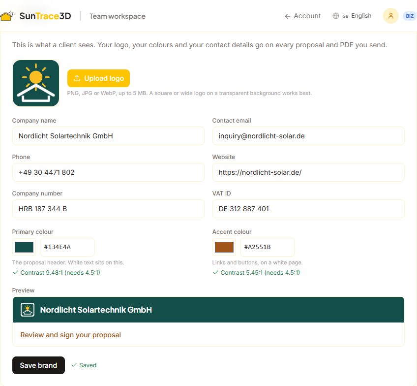
Your brand, not ours
Proposals, PDFs and the pages you share with clients carry your logo, your colours and your contact details. We check the contrast of both colours as you pick them, and will not let you save a colour that would make the text on it unreadable.
Seats, and who is actually in
Professional includes five seats and Enterprise is unlimited. An invite occupies a seat from the moment you send it, so the count always tells you how many people can be added rather than how many happen to have clicked the link already.
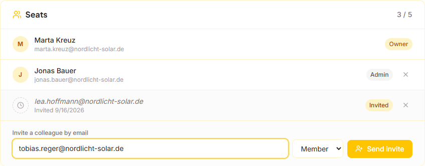
Sharing designs with your team
Designs stay private by default, including the ones you saved before you had a workspace. Share one and everyone with a seat can open and edit it; only its owner can delete it or make it private again. In the project panel, a design belonging to a colleague is labelled with their name, so you can always tell your work from theirs.
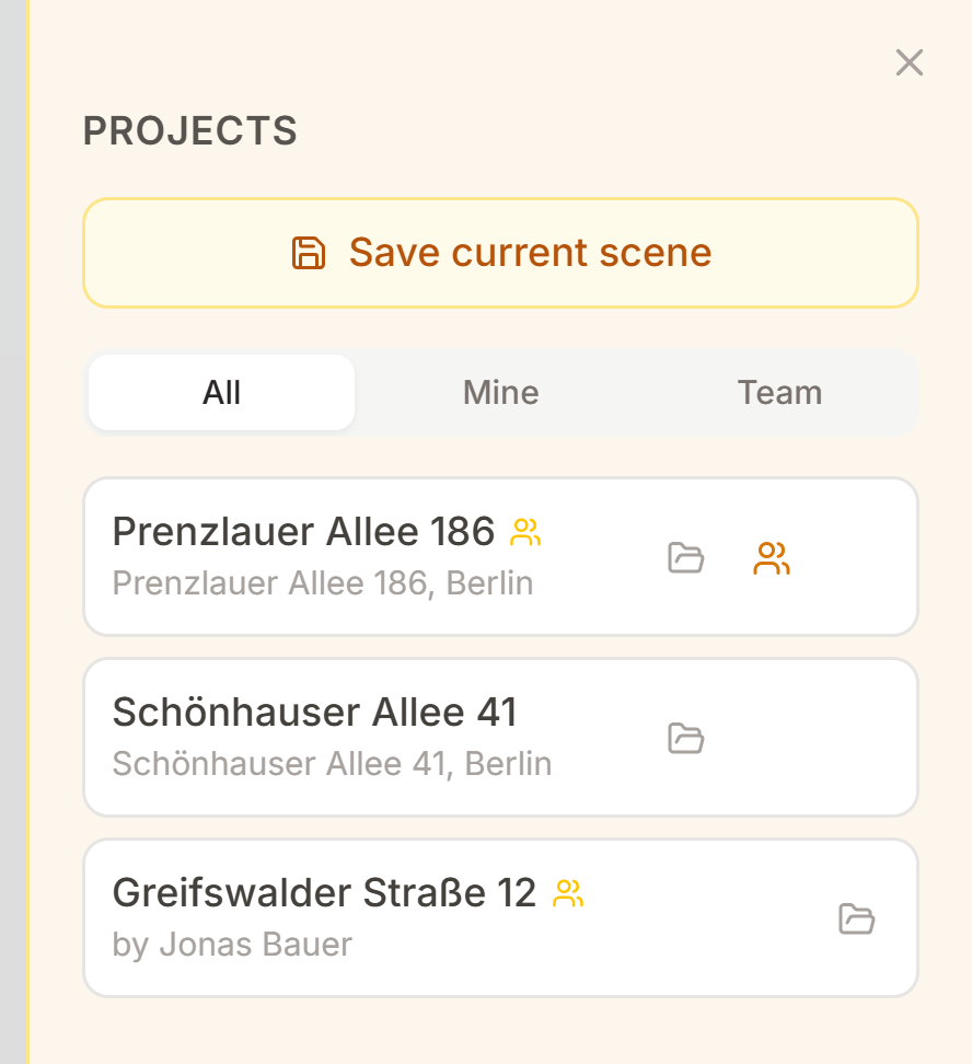
What each role can do
| Role | Can |
|---|---|
| Owner | Everything: company details, brand, seats, and sharing or deleting their own designs. The owner is the account the subscription belongs to. |
| Admin | Change company details and brand, and invite or remove colleagues. Cannot delete designs belonging to someone else. |
| Member | Open and edit every design the team has shared, and create their own. Cannot change company settings or manage seats. |
Tip
Move your existing designs in from the Shared designs card on the workspace page. It only moves designs you own, and you can make any of them private again afterwards from the project panel.
A proposal is a page your client opens from an email — on a phone, usually — showing the system, the price and what it saves, in your brand rather than ours. It carries the same figures as the PDF quote, and the client can accept it there and then. Available on Professional and Enterprise.
Sending a proposal
- 1Set your brand onceGo to Account, then Team workspace, and fill in your logo, colours and contact details. Every proposal you send afterwards uses them.
- 2Design the system and open ReportPlace the panels as usual, then open the report panel and choose Proposal instead of Full report or Quote. The prices, warranties and payment terms are the same fields you already fill in for a quote.
- 3Add the client and create itEnter the client name and email. Creating the proposal freezes the figures and renders the PDF — after this, changing the design does not change what the client sees.
- 4Send it, or copy the linkSend to client emails it for you. You can also copy the link and send it yourself, which is what to do when the client prefers WhatsApp or you want to hand it over in person.
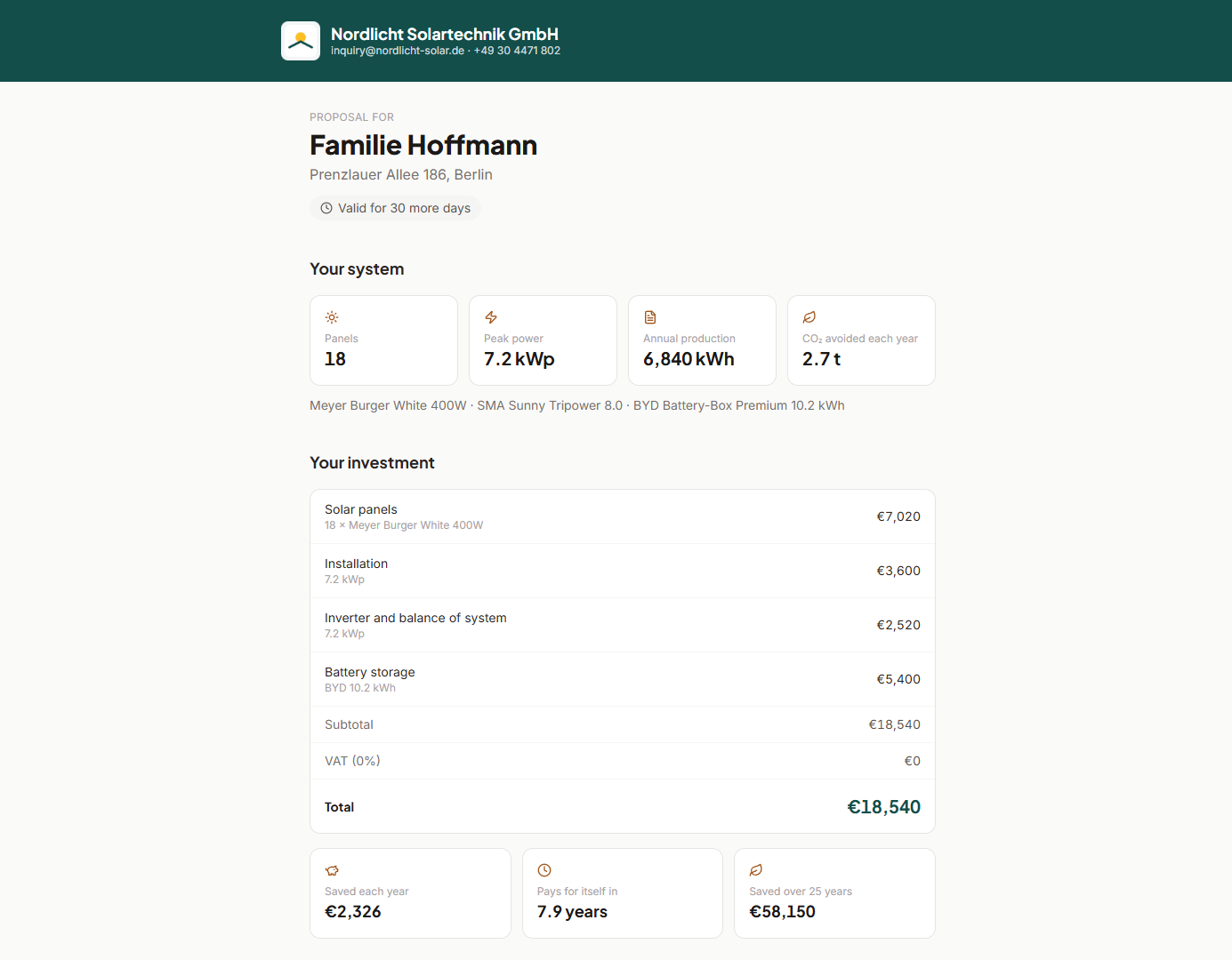
Your brand, on every page
The header, the total and the sign button all take your colours. The PDF matches, and carries your company number and VAT ID in its footer.
Frozen at the moment you send it
A proposal is a snapshot, not a live view. If you change the design tomorrow, the client still sees exactly what you sent — which is also what makes a signature mean something. To offer different figures, send a new proposal.
Staying in control of what you sent
Every proposal expires after the validity period you set, and an expired one stops showing its price. You can revoke a link at any time before it is signed, after which it shows nothing at all. You can also set a passcode, which the client must enter before the proposal opens.
Tip
You can see whether a client has opened a proposal, and when. If the link has not been opened after a few days, the email may have gone to spam — copy the link and send it another way rather than resending the same mail.
A client accepts a proposal by signing it on the page — drawing a signature with a finger or mouse, or typing their name. Both of you receive the signed PDF immediately, with a certificate page recording what was signed and by whom.
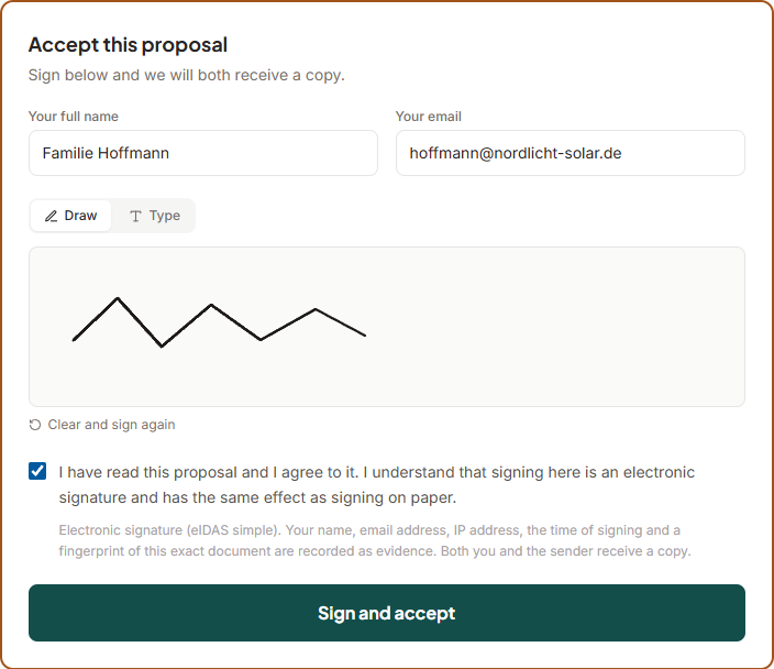
What this signature is, and what it is not
This is a simple electronic signature under Regulation (EU) 910/2014 (eIDAS), Article 25(1). A signature of this kind is admissible as evidence across the EU and cannot be denied legal effect merely because it is electronic. It is the same class of signature used by the other major solar proposal platforms.
It is not an advanced (AdES) or qualified (QES) electronic signature. Those require a qualified trust service provider and identity verification that we do not perform. We will never describe this signature as qualified or certified, and neither should you when talking to a client.
Some contracts carry a statutory written-form requirement that a simple electronic signature does not satisfy — certain consumer construction contracts in Germany among them. Where that applies to the work you sell, treat a signed proposal as a clear record of acceptance and follow it with whatever form the law requires.
What gets recorded
A simple electronic signature carries no cryptographic identity, so its weight comes entirely from the record kept around it. That record is printed on the certificate page of the signed PDF and stored with the proposal.
| Recorded | Why it matters |
|---|---|
| Name and email | Who said they were accepting, and where they can be reached. |
| Time of signing (UTC) | When acceptance happened, in a timezone that cannot be argued about. |
| IP address | Where the signature came from. Recorded as unknown rather than guessed if it cannot be determined. |
| The exact consent wording | Stored word for word, in the language the signer read, along with a version marker. The wording changes between releases; what matters is what this signer agreed to. |
| A fingerprint of the document (SHA-256) | Identifies the exact file that was signed. Change one character of the proposal and the fingerprint no longer matches, so "this is what was signed" is a fact anyone can check rather than something you have to take our word for. |

Tip
A proposal can only be signed once. If a client signs and then wants changes, send a new proposal rather than reopening the old one — the signed copy stays as the record of what was agreed the first time.
Sharing a design for review used to end in a conversation. A client could pin comments on the model and then there was nothing to press — no way to say yes, and no way for you to find out that someone was waiting on you. Now a review ends in an answer, and an approved one hands the client straight to signing your proposal.
The loop end to end
- 1Share the design, and send a proposal with itCreate the review session as usual, then create a proposal for the same design. They link themselves — the proposal offers the client a way to walk the model in 3D, and approving the review takes them to the proposal.
- 2Your client looks, and answersThey pin comments where they want them, then either approve or ask for changes. Either answer emails you.
- 3You see what is waiting in one placeAccount, then Team workspace, then Client reviews. Every design you have shared, with how many comments are still unanswered on each.
- 4Change the design and send an updateEdit the saved design, then press Send an update on that review. Your client gets an email, and the review reopens on the new version.
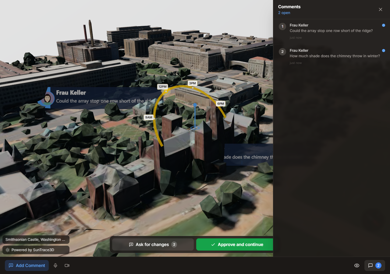
Approve and continue
Closes the review and, if a proposal is attached, opens it at the signature. The client says yes and signs in the same minute, instead of going to look for an email. Approval is final: a client who then wants changes needs a new review.
Ask for changes
Keeps the review open and puts it at the top of your inbox with the number of comments waiting for an answer. Your client sees that the message got through.
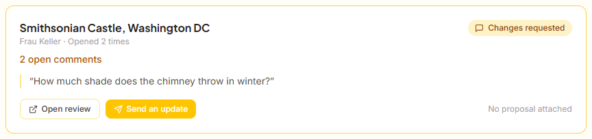
Versions, and why old comments stay
Sending an update bumps the review to the next version and reopens it. The earlier comments are not deleted — they are marked against the version they were written about, and shown as answered. Deleting them would erase the record of why the design changed; quietly re-labelling them would be worse, because a pin that said "move this panel" would look like it was pointing at the panel that replaced it.
Tip
Send the proposal at the same time as the review, not after it. The value of Approve and continue is that there is something to continue to — without a proposal attached, approving simply closes the review and you still have to follow up.
Engineering & Design
Professional-grade PV system design tools: equipment selection, string planning, electrical diagrams, cable sizing, consumption analysis, battery simulation, and data export.
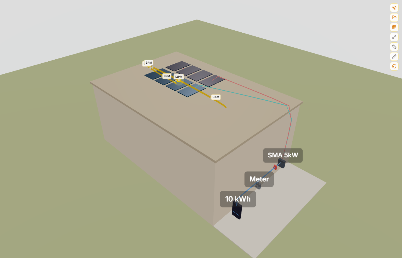
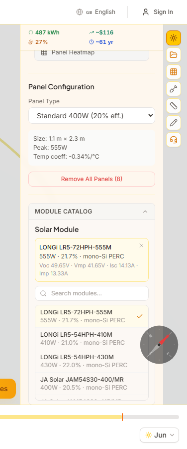
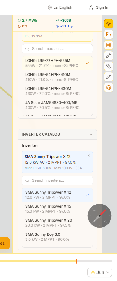
SunTrace3D includes a built-in catalog of real CEC-certified solar modules and inverters from leading manufacturers such as LONGi, JA Solar, Canadian Solar, SMA, Fronius, and more. Select specific equipment to unlock accurate string planning, cable sizing, and energy analysis based on real electrical specifications.
How to Use
- 1Open the Module CatalogIn the solar sidebar, expand the 'Module Catalog' section. A searchable list of solar modules appears with manufacturer, model, wattage, and efficiency.
- 2Select a moduleClick any module to select it. A summary card shows the full electrical specifications: open-circuit voltage (Voc), max power voltage (Vmp), short-circuit current (Isc), max power current (Imp), and temperature coefficients.
- 3Choose an inverterExpand the 'Inverter Catalog' section and select an inverter. The summary shows MPPT count, voltage range, maximum input voltage, rated AC output, and European efficiency.
Module and inverter selections are saved with your project. When you load a saved project, the equipment choices are automatically restored.
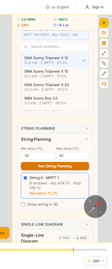
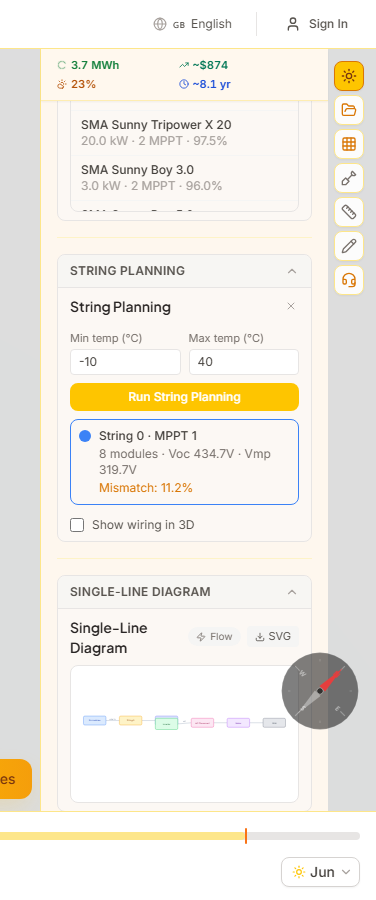
String planning automatically groups your solar panels into electrical strings based on temperature-corrected voltage limits, shading similarity, and panel orientation. The algorithm respects inverter MPPT input constraints and generates warnings when voltage or current limits are violated.
How to Use
- 1Select equipment firstChoose a module and inverter from the catalogs. The string planner needs their electrical specifications (Voc, Vmp, MPPT ranges) to compute valid string configurations.
- 2Set design temperaturesEnter the minimum and maximum expected temperatures for your location. These are used to calculate temperature-corrected Voc (cold) and Vmp (hot) voltages that determine safe string lengths.
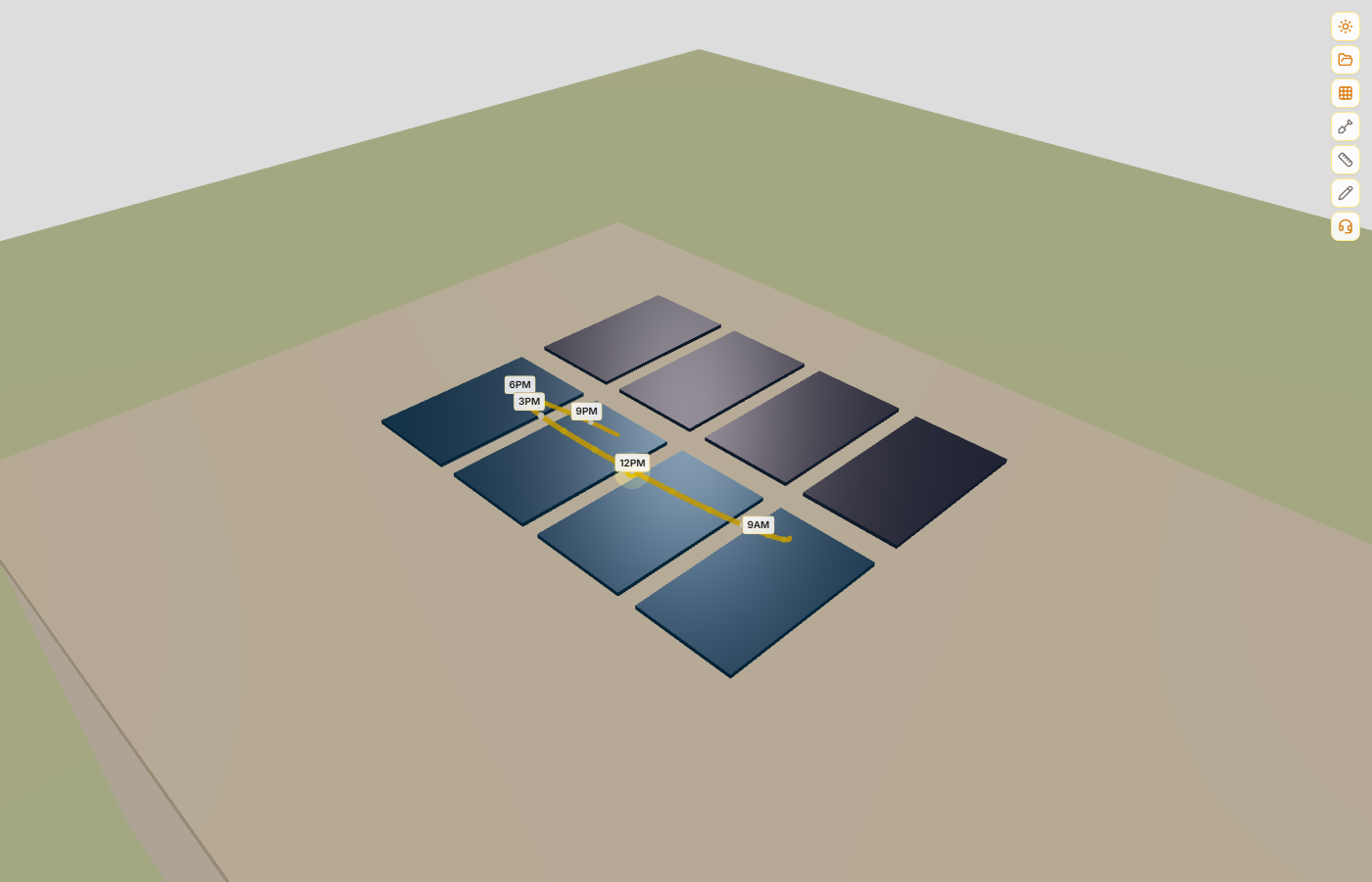
- 3Run planningClick 'Run Planning'. The algorithm clusters panels by orientation and shading profile, then packs them into strings that stay within the inverter's voltage window. Each string is assigned a distinct color.
- 4Review resultsEach string card shows module count, temperature-corrected Voc and Vmp, estimated mismatch loss, and MPPT assignment. Warnings appear if any string exceeds inverter limits.
Panels in the 3D viewer are color-coded by string group, making it easy to visually verify the grouping.
The single-line diagram (SLD) is an auto-generated electrical schematic of your PV system. It shows the flow from module groups through strings and MPPT inputs to the inverter, AC disconnect, meter, and grid connection — the standard format required for permit applications.
How to Use
- 1Complete string planningThe SLD is generated automatically once a valid string plan exists. It reads the string configuration, MPPT assignments, and inverter specifications.
- 2View the diagramExpand the 'Single-Line Diagram' section. The SVG diagram shows module groups on the left, connected through strings to MPPT inputs, then to the inverter, AC disconnect, meter, and grid.
- 3Download as SVGClick the SVG button to download the diagram as a vector file. This can be included in permit applications or engineering documentation.
The SLD is automatically included in PDF site reports when you generate one.
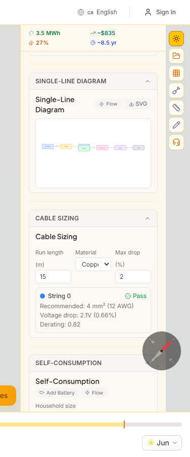
Cable sizing calculates the recommended conductor cross-section for each DC string run, ensuring voltage drop stays within the allowable limit (typically 2%). It supports both copper and aluminum conductors and accounts for derating factors.
How to Use
- 1Enter cable run lengthsFor each string, enter the one-way cable length in meters from the panels to the inverter. If you have measurements from the Measure Tool, these can be used as reference.
- 2Select conductor materialChoose between copper (lower resistance, standard residential) or aluminum (lighter, common in commercial installations).
- 3Review recommendationsThe calculator shows the recommended cable size in mm² and AWG, the calculated voltage drop in both volts and percentage, and a clear Pass/Fail indicator against the maximum allowable drop.
The voltage drop formula uses Vdrop = 2 x I x L x resistivity / area, iterating through standard cross-sections until the drop is within limits.
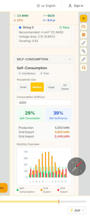
Self-consumption analysis models the interaction between your solar production and household electricity usage throughout the year. It calculates how much solar energy you consume on-site versus export to the grid, using realistic hourly load profiles based on household size.
How to Use
- 1Select a household presetChoose from four load profiles: Small (2,500 kWh/year), Medium (4,500 kWh/year), Large (6,500 kWh/year), or EV Owner (8,500 kWh/year). Each has a realistic hourly consumption shape with morning and evening peaks.
- 2Adjust annual consumptionFine-tune the total annual consumption in kWh. The hourly profile shape stays the same but scales to match your target.
- 3Read the resultsTwo key metrics are displayed: Self-Consumption (percentage of solar production used on-site) and Self-Sufficiency (percentage of total consumption covered by solar). A monthly stacked bar chart shows the breakdown of self-consumed, exported, and imported energy.
Higher self-consumption means more value from your solar investment. Adding battery storage (see next section) significantly increases self-consumption by storing daytime surplus for evening use.
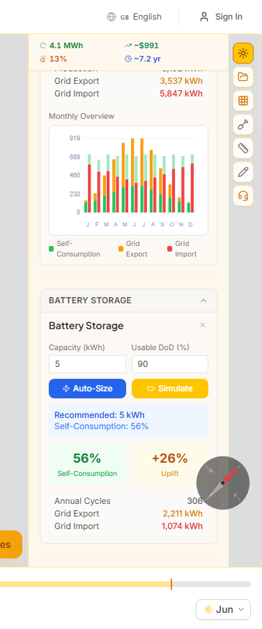
Battery storage simulation models how a home battery system changes your self-consumption and grid dependence. It includes an auto-sizing recommendation that finds the optimal capacity based on your production and consumption patterns.
How to Use
- 1Auto-size the batteryClick 'Recommend' to run a capacity sweep from 1 to 20 kWh. The algorithm finds the knee point where adding more capacity yields diminishing returns in self-consumption improvement.
- 2Or configure manuallyEnter a specific battery capacity in kWh and click 'Simulate'. You can also adjust depth of discharge, round-trip efficiency, and max charge/discharge power for detailed modeling.
- 3Compare with and withoutResults show the new self-consumption and self-sufficiency percentages with battery, the uplift compared to no-battery, estimated annual charge/discharge cycles, and updated grid import/export figures.
The greedy dispatch algorithm charges the battery with surplus solar during the day and discharges during evening peak consumption. Round-trip efficiency losses (typically 8-10%) are accounted for in all calculations.
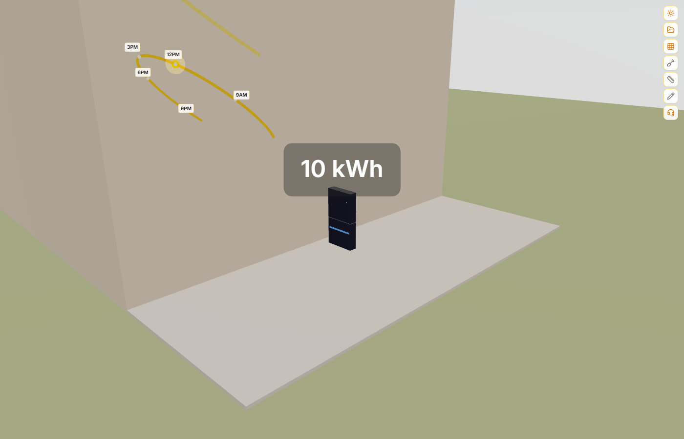
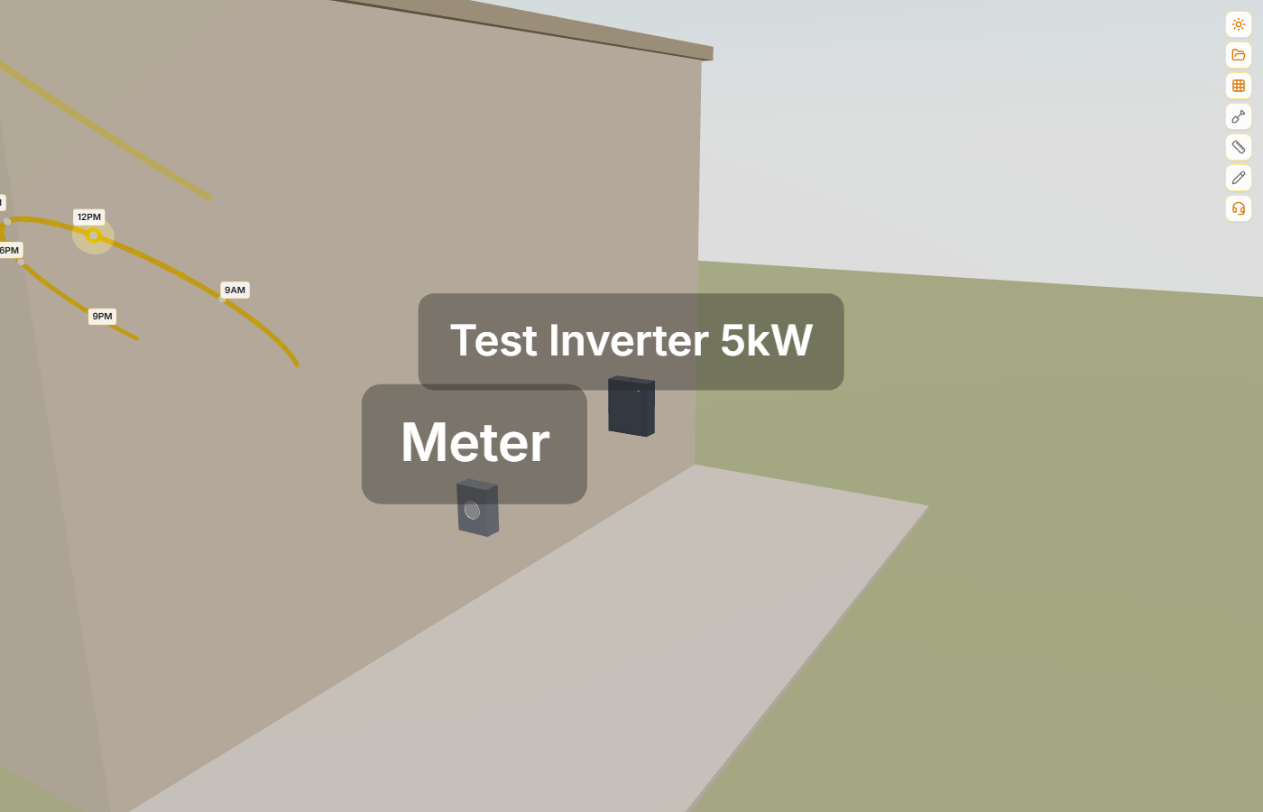
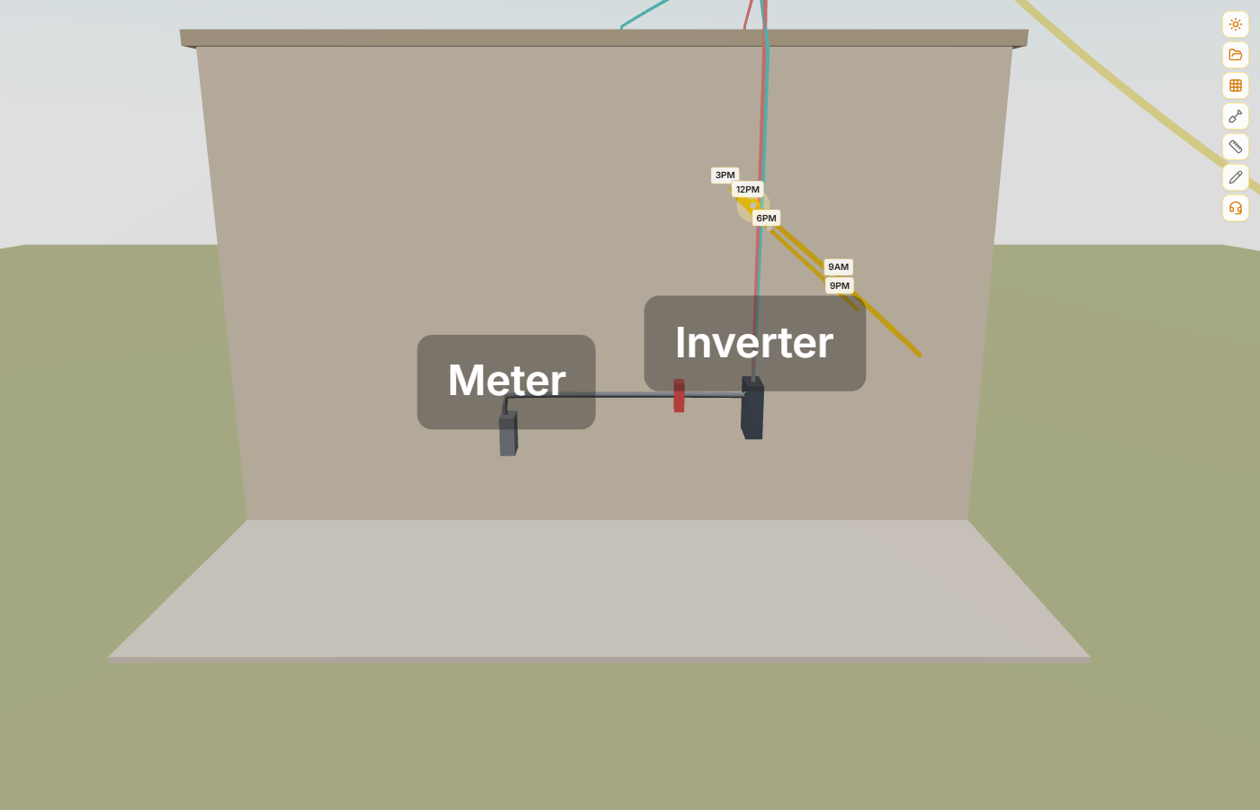
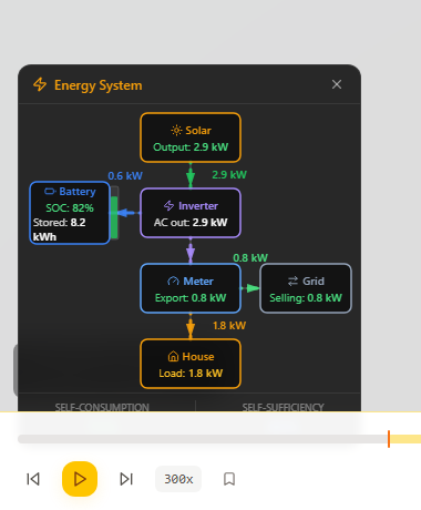
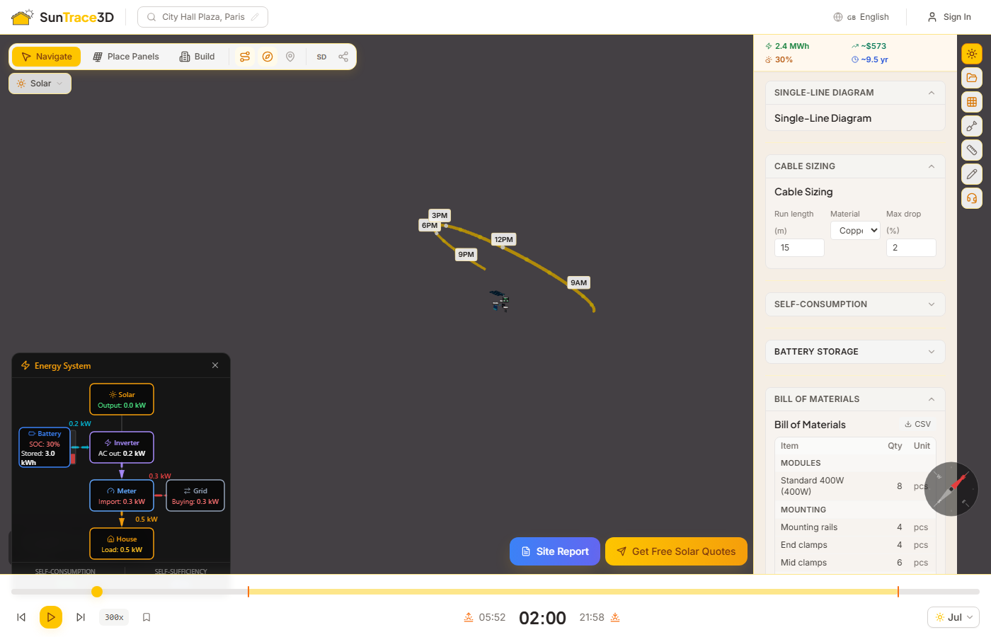
The Energy System Dashboard is a real-time 2D overlay that shows how electricity flows between your solar panels, inverter, battery, meter, and house. It appears automatically when you run a self-consumption analysis and updates live as you scrub the time slider. Click any component to fly the 3D camera to that object in the scene.
How to Use
- 1Run self-consumption analysisPlace solar panels, add an inverter and meter, then run the self-consumption analysis from the engineering sidebar. The dashboard appears automatically.
- 2Read the live energy flowsThe dashboard shows real-time power values (kW) for solar production, battery charge/discharge, grid import/export, and house consumption. Animated arrows indicate the direction of energy flow between components.
- 3Click to navigateClick any component box (Solar, Inverter, Battery, Meter, House) to fly the 3D camera to that object in the scene. The camera zooms in close enough to inspect the equipment.
- 4Scrub the time sliderMove the time slider to see how energy flows change throughout the day. At noon, solar production peaks and excess charges the battery or exports to grid. At night, the battery discharges and the grid supplies remaining demand.
Real-Time Monitoring
Live power values update as you move the time slider. See solar production, battery state of charge, grid import/export, and house consumption at any time of day.
Click to Navigate
Each component in the schematic is clickable. Click Solar to fly to the panel array, click Battery to zoom to the storage unit, or click Meter to inspect the grid connection.
The dashboard also shows summary metrics — self-consumption percentage (how much solar you use directly) and self-sufficiency percentage (how much of your demand is met by solar + battery). On mobile devices, the dashboard automatically switches to a compact grid layout.
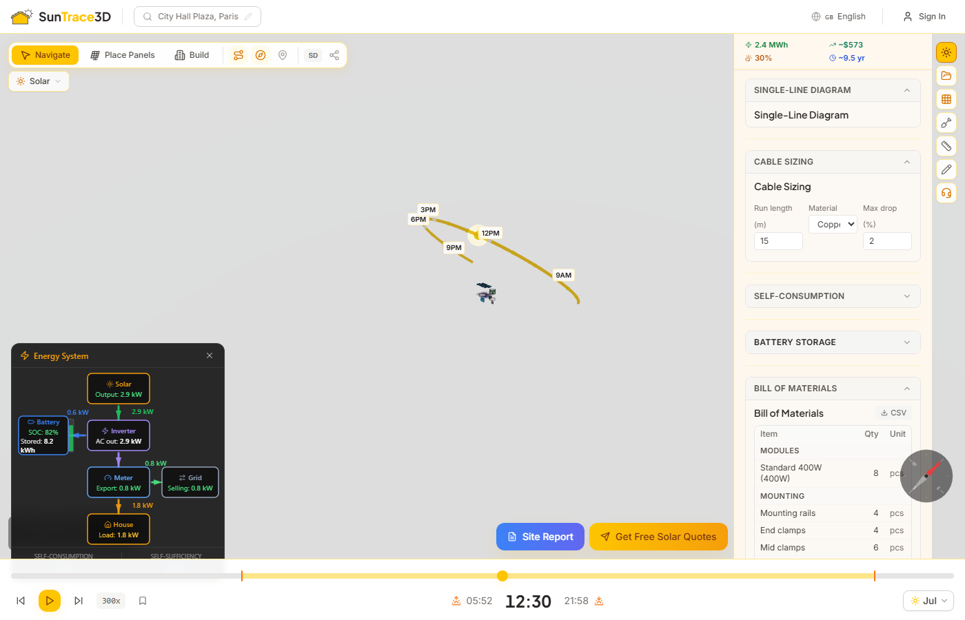
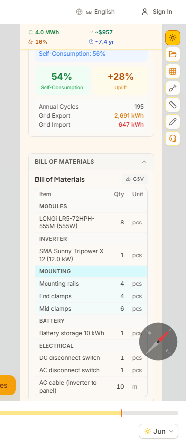
The Bill of Materials aggregates all components needed for your PV installation into a single table. It includes modules, inverter, mounting hardware, DC and AC cables, disconnects, and optional battery — providing a quick material checklist for procurement.
How to Use
- 1Automatic generationThe BOM is generated automatically from your panel layout, selected equipment, string plan, and cable sizing results. No manual input needed.
- 2Review line itemsThe table groups items by category: modules, inverter, mounting (rails and clamps), cable (per cross-section from cable sizing), battery (if configured), and electrical components (DC and AC disconnects).
- 3Export to CSVClick the CSV button to download the complete bill of materials as a spreadsheet-compatible file for import into procurement or ERP systems.
The BOM is also included in PDF site reports. Mounting hardware quantities are estimated using standard heuristics: 2 rails per panel row, clamps at each panel edge plus shared mid-clamps.
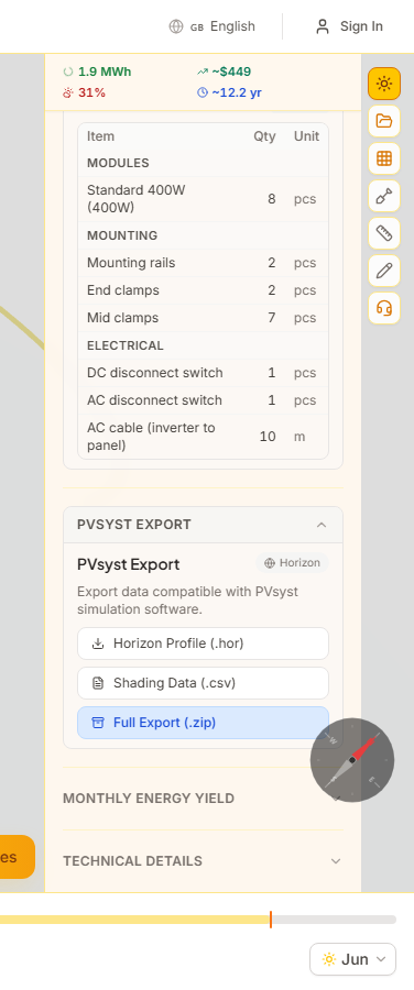
Export your shading analysis data in PVsyst-compatible formats for detailed simulation in external software. Three export options are available: a horizon profile (.hor), a per-panel shading summary (.csv), and a comprehensive ZIP archive containing all data files.
How to Use
- 1Download horizon profileThe .hor file contains azimuth-elevation pairs describing the horizon obstruction profile as seen from the center of your panel array. This is the standard input format for PVsyst near-shading analysis.
- 2Download shading CSVThe .csv file lists each panel with its tilt, azimuth, shading loss percentage, and annual yield estimate. If string planning has been run, the string assignment is included.
- 3Download full export ZIPThe comprehensive ZIP archive bundles all export files: system summary, panel layout with per-panel kWh, monthly yield data, string configuration, horizon profile, and shading analysis. This is the recommended option for a complete PVsyst import package.
The horizon profile is computed by casting rays from the array centroid at 5-degree azimuth steps across the full 360-degree range, finding the highest obstruction elevation angle at each step.
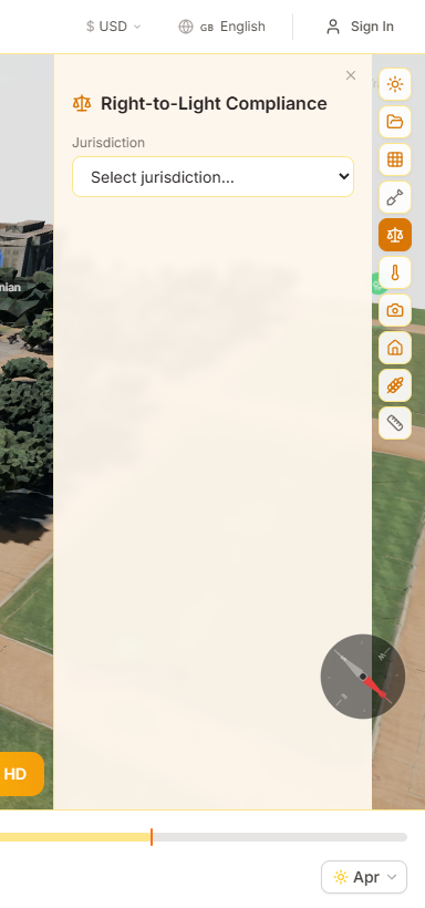
The Right-to-Light panel helps architects and urban planners assess whether a proposed development meets daylight access standards. Based on BRE 209 (Site Layout Planning for Daylight and Sunlight), it analyzes how much skylight and sunlight reaches neighboring windows.
How to run a compliance check
- 1Switch to the Compliance verticalSelect 'Right-to-Light' from the industry dropdown in the top-left corner of the viewer.
- 2Add windows to analyzeClick on building facades to place window markers. Each window is checked against BRE 209 vertical sky component (VSC) and annual probable sunlight hours (APSH) thresholds.
- 3Review compliance indicatorsWindows are color-coded: green (passes), amber (marginal), red (fails). The sidebar shows detailed metrics for each window.
- 4Generate a compliance reportExport a PDF report with window-by-window analysis, compliance status, and 3D visualizations for planning submissions.
Vertical Sky Component (VSC)
VSC measures the amount of visible sky from a window point. BRE 209 recommends a minimum of 27% VSC for adequate daylight. Windows below this threshold are flagged.
Annual Probable Sunlight Hours (APSH)
APSH measures the percentage of annual sunlight hours a window receives compared to an unobstructed location. BRE 209 recommends at least 25% annual and 5% winter APSH.
Best practice
Run compliance checks early in the design process. Small changes to building height, setback, or orientation can significantly improve daylight access to neighboring properties.
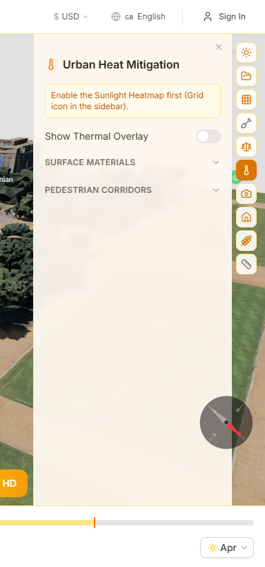
The Urban Heat panel maps thermal exposure across urban areas. It analyzes how shade coverage, surface materials, and building geometry affect surface temperatures and pedestrian thermal comfort.
How to analyze urban heat
- 1Switch to the Thermal verticalSelect 'Urban Heat' from the industry dropdown in the viewer toolbar.
- 2Enable the thermal overlayToggle the heat map overlay to see color-coded surface temperature estimates across the scene, based on shade coverage and material albedo.
- 3Analyze pedestrian corridorsMark pedestrian paths to see shade coverage along walking routes. The panel shows the percentage of each corridor that is shaded during peak heat hours.
Material Albedo
Different surfaces absorb and reflect heat differently. The material palette lets you assign albedo values (reflectivity) to roofs, pavements, and green spaces to model their thermal impact.
Thermal Comfort Zones
The heat map identifies areas of thermal stress based on combined sun exposure, shade coverage, and wind exposure. Red zones indicate areas where pedestrians may experience heat discomfort during summer.
Mitigation strategies
Use the scene objects tool to add trees and shade structures, then re-run the thermal analysis to see their cooling effect. Even small increases in shade coverage can significantly reduce surface temperatures.
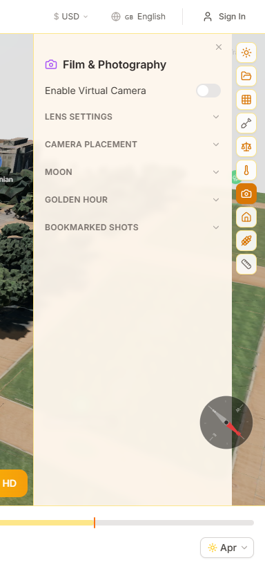
The Film & Photography panel provides tools for planning shoots around natural light. Calculate golden hour and blue hour times, preview camera angles through virtual lenses, and bookmark lighting setups for location scouting.
How to plan a shoot
- 1Switch to the Camera verticalSelect 'Film & Photo' from the industry dropdown in the viewer toolbar.
- 2Check golden hour timesThe sidebar shows exact golden hour and blue hour start/end times for the current date and location. Use the date picker to plan for future shoot dates.
- 3Place a virtual cameraClick the camera placement button and click in the scene to position a virtual camera. Choose a focal length (24mm–200mm) to preview the frame.
- 4Bookmark your setupSave camera positions and lighting conditions as bookmarks. Jump between scouted viewpoints when comparing angles or planning multi-camera setups.
Lens Simulation
The virtual camera previews the field of view for common focal lengths: 24mm (wide), 35mm (street), 50mm (standard), 85mm (portrait), and 200mm (telephoto). The preview updates in real-time as you reposition the camera.
Moon Position
For night scene planning, the moon tracker shows moonrise, moonset, and current position. Useful for planning moonlit exterior shots or understanding ambient light conditions after sunset.
Location scouting workflow
Search your location, set the date to your planned shoot day, scrub through the time slider to find the best lighting window, place your camera, and save the bookmark. On shoot day, reload the project to reference your planned angles.
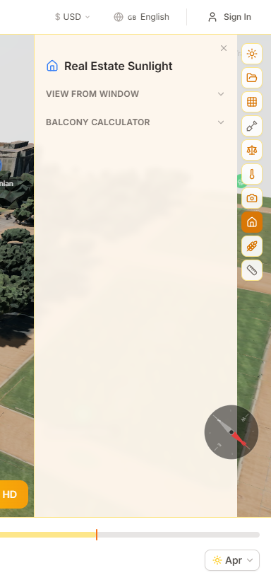
The Real Estate panel provides tools for showcasing property sunlight exposure. Analyze window views, calculate balcony sun hours, and generate solar scores that quantify a property's energy potential for buyers.
How to analyze a property
- 1Switch to the Real Estate verticalSelect 'Real Estate' from the industry dropdown in the viewer toolbar.
- 2Run a window view analysisClick on windows to preview the view from inside. The panel shows what residents will see, including surrounding buildings, vegetation, and sky exposure.
- 3Calculate balcony sun hoursMark balcony positions to see how many hours of direct sunlight they receive across different seasons. Great for marketing south-facing apartments.
- 4Generate a property sun scoreThe solar score summarizes total sun exposure, shade risk, energy potential, and environmental benefits in a single shareable metric for property listings.
Window View Preview
The view-from-window feature renders what residents will actually see from each window. This helps buyers understand sight lines, privacy, and natural light before visiting the property.
Balcony Calculator
The balcony calculator shows monthly direct sunlight hours for any outdoor space. Summer vs. winter comparison helps buyers understand seasonal sun exposure for balconies, terraces, and patios.
Listing enhancement
Include the property's solar score and sunlight metrics in your listing description. Properties with quantified sun exposure data generate more interest and can justify higher asking prices.
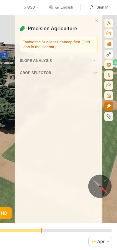
The Agriculture panel provides tools for planning crop placement and greenhouse positioning based on actual sunlight data. Map sun exposure across your land, check crop suitability, and model light levels inside greenhouses.
How to plan your farm layout
- 1Switch to the Agriculture verticalSelect 'Agriculture' from the industry dropdown in the viewer toolbar.
- 2Enable the sunlight heatmapToggle the heatmap to see color-coded sun exposure across your land. Use the monthly view to track seasonal changes from planting through harvest.
- 3Check crop suitabilityOpen the crop selector and choose a crop type. The suitability map highlights which areas of your property match the crop's sunlight and climate requirements.
- 4Configure greenhousesPlace greenhouses in the scene, set glass transmission (30–95%), and see realistic interior light levels on the heatmap. Position them for maximum growing-season sunlight.
Slope & Aspect Analysis
The terrain analysis shows slope angle and aspect direction across your property. South-facing slopes receive more sunlight, while steep north-facing slopes may be unsuitable for sun-loving crops.
Crop Suitability System
Select a crop from the database (50+ species) to see a color-coded suitability map. Green zones have ideal sunlight and climate conditions, amber zones are acceptable, and red zones are unsuitable for that crop.
Seasonal planning
Use the monthly heatmap to compare spring vs. summer sun exposure. Areas that get full sun in July may be partially shaded in April when you're starting seedlings — plan your layout around growing-season sunlight, not just midsummer.
The Live Events vertical helps event planners, festival producers, and venue managers design outdoor event layouts with accurate sun and shade simulation. Position stages, seating, tents, and production equipment in 3D, then scrub through the timeline to see exactly where shadows fall during every hour of the event.
How to plan an event layout
- 1Switch to the Live Events verticalSelect 'Live Events' from the industry dropdown in the viewer toolbar, or visit the live events landing page and click 'Try it now.'
- 2Enter Build modeClick Build, then select the Events tab. Choose from 8 asset types: Pop-up Tent, Stage, Chair, Dining Table, Speaker Stack, LED Wall, Lighting Truss, or Barrier.
- 3Place and configure assetsAdjust width, depth, and height with sliders. Pick a color from the swatch palette (white, black, wood, gold, red). Click on the ground or on another object to place.
- 4Stack objectsPlace speakers on a stage or lights on a truss. Stacked objects automatically move and rotate with their parent when repositioned.
- 5Check shadows throughout the dayUse the time slider to scrub through the event day. Add timeline bookmarks at key moments (ceremony start, reception, golden hour) for quick comparison.
8 Event Asset Types
Pop-up tents, stages, chairs, dining tables, speaker stacks, LED walls, lighting trusses, and barriers — each with adjustable dimensions and color palette.
Shadow Planning for Events
Identify guest comfort issues, stage glare risk, and screen washout before the event day. Use timeline bookmarks to save key moments for quick reference.
Object stacking
Speakers placed on a stage, lights hung from a truss, or any object placed on another object will automatically move and rotate together. Delete the parent to remove all attached children.
The CRM Platform lets solar professionals and businesses manage territories, detect rooftop prospects automatically, and run targeted outreach campaigns — all from within SunTrace3D. Draw a polygon on the map, and the system scans every building inside it, scores their solar potential, and presents them in a sortable prospect grid. Available on Business plans and above; a free playground lets anyone try it with limited results.
How to use the CRM
- 1Access the CRMNavigate to the CRM section from the main menu. Business and Enterprise subscribers see the full CRM app. Free and Pro users can try the interactive playground, which scans a small area and reveals details for up to 3 prospects.
- 2Draw a territoryClick on the map to draw a polygon boundary around your target area. The system calculates the polygon area and validates it against your plan's territory size limit. Once confirmed, a region scan begins automatically.
- 3Review detected prospectsThe scan detects every building within your territory using satellite-derived footprints, classifies them by type (residential, commercial, industrial), estimates usable roof area, and calculates a solar score based on panel count, annual yield, and local climate data. Results appear in a sortable, filterable grid.
- 4Create campaignsSelect prospects and create outreach campaigns with personalized materials — mail templates, email content, and print assets with QR codes. Each QR code tracks engagement and automatically advances the prospect through your sales pipeline.
- 5Track results on the dashboardThe CRM dashboard shows your sales funnel, territory potential in kWp, recent activity, and conversion metrics. Data refreshes automatically so you always have the latest picture of your pipeline.
Territory Scanning
Building detection uses satellite-derived footprint data to find every building in your territory. Each one is automatically classified, measured, and scored without any manual data entry.
Solar Scoring
Each prospect receives a solar grade (A+ to D) based on estimated roof area, panel capacity, annual energy yield, and local irradiance. Scores help you prioritize the highest-value opportunities.
Industry Verticals
The CRM supports multiple industry verticals from a single workspace. Each vertical brings its own enrichment fields, scoring logic, pipeline stages, and grid columns. Switch verticals per campaign — a single customer can have both rooftop solar and real estate campaigns.
Real Estate Vertical
Score properties by sun exposure, estimate property values from country-level price defaults, calculate neighborhood amenity proximity (schools, transit, parks, shops), and compute real estate commissions. Each prospect shows living area, estimated floors, year built, and a 100-point amenity score.
Prospect Journey & Pipeline
Track each prospect through a 10-stage pipeline from Identified to Installed. The journey drawer shows an append-only activity timeline — every stage change, note, and QR scan is logged. Edit stages inline from the prospect grid, or let QR code scans auto-advance the journey.
Real-Time Dashboard
The CRM dashboard shows your funnel by stage, remaining territory potential in kWp that shrinks as prospects convert, campaign performance metrics, and a live activity feed. Data refreshes automatically every 30 seconds so you always see the latest pipeline state.
Interactive Territory Map
Draw polygon boundaries on an interactive map with click-to-draw tools. Building footprints render on a canvas overlay with choropleth coloring — shade prospects by solar grade, deal value, or pipeline stage. Click any footprint to open the prospect detail.
Free Playground
Anyone can try the CRM without signing up at /crm. Draw a small region (up to 0.25 km²) and the system scans every building, scores solar potential, and reveals full details for 3 sample prospects. The rest are blurred with an upgrade prompt — no account required to explore.
It ends in a signature
A scanned roof opens as a real design, the design becomes a branded proposal, and the signature closes the deal — each step moving the prospect along its pipeline by itself.
Section 67 follows one roof the whole way: from a pin on a territory map to a signed contract and a number on the dashboard.
The CRM automatically detects every building in your territory, classifies it by type, and scores its solar potential — no manual data entry required.
Scanning a territory tells you which roofs are worth a visit. This is the part where one of them becomes a customer. Opening a scanned roof as a design creates a real project in your workspace, seeded with what the scan already measured, and carries the prospect with it — so the proposal you produce at the end belongs to that person, and the CRM knows it happened without anyone updating a card.
From a scanned roof to a signed contract
- 1Open the roof as a designIn the prospect drawer, press Design this roof. A project is created for your workspace, named after the address and shared with your team, and the prospect moves into the pipeline. Pressing it again re-opens the same design rather than creating a second one — two designs for one roof would be two places to make every change.
- 2Design from what the scan already knowsThe viewer opens on that roof with a banner naming the prospect, the stage and the estimated value. Open the solar wizard and the territory scan’s own estimate is waiting there: the panel count it found, and a monthly usage target already filled in. Change anything you like — the scan is a starting point, not an answer.
- 3Turn the design into a proposalCreate proposal in the banner opens the proposal form with the client already named, in your company’s branding, with your standard terms and warranties. It is the same proposal described in section 64 — it simply knows which prospect it is for.
- 4Send itSending moves the prospect to the stage your vertical calls quoted and sets its deal value to the proposal total, to the cent. Nothing else needs doing.
- 5They signA signature closes the loop: the prospect moves to won, the signed PDF and its signature certificate are stored, and the dashboard counts it. The journey now reads as a record of what happened rather than a status somebody remembered to set.

The scan is your starting point
Panel count, capacity and annual yield come from the territory scan, so the wizard opens on the numbers that made you visit this roof instead of an empty form.
A scan is not permission to write
The client email is never filled in for you from a scanned contact, and a proposal cannot be sent without an address you entered. Under GDPR, a roof appearing in a scan is not consent to be contacted — and a signed proposal is not consent to be marketed to.
What moves a prospect, and where
Each vertical names these milestones in its own language, so shared code never has to know that an installer says quoted and an estate agent says offer. Movement is forward only: a proposal sent after one was already signed will not drag a won deal backwards, and a prospect somebody marked lost or do-not-contact is left where they put it.
| What happened | Solar installer | Estate agent |
|---|---|---|
| A design was opened for the roof | Site assessment | Viewing |
| A proposal was sent | Quoted, with the proposal total as the deal value | Offer, with the proposal total as the deal value |
| The client signed | Won | Sold |
| The client declined | Lost | Lost |
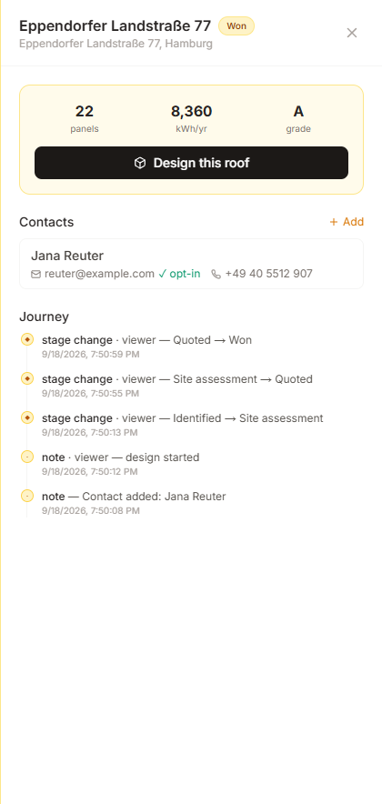
Potential, and what came of it
Every figure the dashboard could show used to be an estimate of what a territory might be worth, which made it impressive and impossible to check. The Realised block is the other half: proposals sent, proposals signed, the conversion rate between them, and the value actually won — each in the currency the proposal was written in. Remaining potential now drops as deals close, so the two halves always agree.
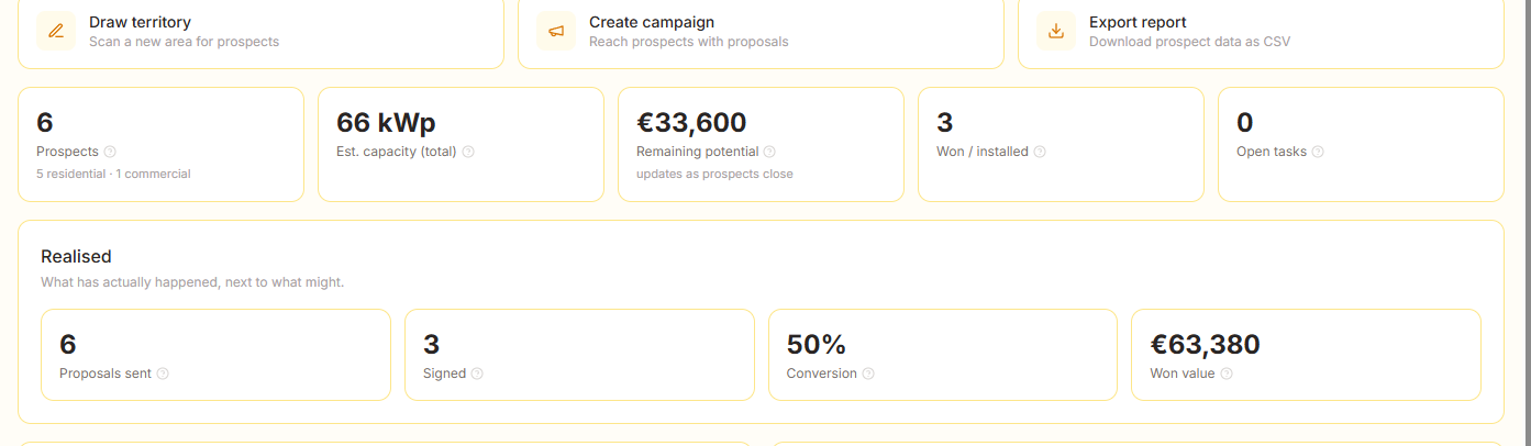
Tip
Stages only ever move forward, and terminal ones (won, lost, do not contact) are left alone by every automatic step. If you mark a prospect lost, opening its design again will not quietly reopen the deal — only you can do that, by moving it yourself.
Regulatory
Country rules, tariffs and filings — Germany first
Germany is the most regulation-dense residential solar market in Europe, and tools built for the US leave the paperwork to you. When a site is in Germany, a Tariffs & Compliance panel appears in the viewer: the feed-in tariff for this system on its commissioning date, the VAT the law puts on it, a grid-connection pre-check, and the registration sheet pre-filled from the design. Everything carries a date and a link to the source it came from.
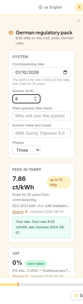
Using the pack
- 1Design the system as usualThe panel appears once the site is in a country we have a pack for, and reads the capacity straight off the panels on the roof. Nothing extra to set up.
- 2Tell it the three things the roof cannotThe commissioning date, which fixes the tariff for twenty years; the inverter rating in kVA and the number of phases, which is what the grid rules are written in; and who will own the plant, which is what the register asks for.
- 3Enter your own rates onceWhere a published rate has gone past its verification date we do not show it — we ask you for yours. Enter it once and it is used for every quote in your workspace, shown as your figure with ours beside it.
- 4Send the proposalA German proposal carries a Compliance and filings section into the page and the PDF: the VAT and its statute, the tariff and its source, the grid standard, the register, and the disclaimer — in German on a German document.
How much to trust a number
Rates change by publication and law changes by amendment, and nobody here is watching either for you. So every figure states its own condition, and the panel refuses to show one it cannot stand behind.
| What you see | What it means |
|---|---|
| A figure with a date | Checked against its source within the last 90 days. The source link is beside it. |
| A figure with an amber warning | More than 90 days since it was last checked. Still shown, with its age, and the same warning goes into the PDF. Verify before you contract. |
| No figure at all | More than 180 days since a market rate was checked: it is withheld rather than quoted, and you are asked for yours. A dead tariff inside a twenty-year payback is wrong for twenty years. |
| A figure marked as yours | Your own value, used everywhere in your workspace, with our last figure and its date shown beside it so any divergence is visible. |
VAT that knows the threshold
§12(3) UStG zero-rates residential PV up to 30 kW (peak). The proposal form applies it automatically and warns when a system is over the line — a quote that stays silently at 0% above it is a tax error you carry.
Registration, pre-filled
Every German plant must be in the Marktstammdatenregister within a month of commissioning. We fill the sheet from the design; you file it. Nothing is submitted automatically and no account of yours is used.
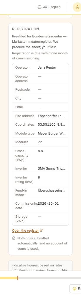
What this is not
Indicative figures to design and quote from, not tax or legal advice, and not a substitute for the current Bundesnetzagentur publications or the legislation in force. No figure here has been reviewed by a German energy lawyer or tax adviser, which is exactly why every one of them carries its source, its date and its own warning.
VDE-AR-N 4105 governs how a generating plant connects to the low-voltage grid. Its limits are easy to miss while a design is still moving — and expensive to discover at the connection appointment. The pre-check compares the design on screen against them and names the clause for each result.
| Check | Limit | Why it matters |
|---|---|---|
| Low-voltage connection | 135 kVA | Above it the plant needs a medium-voltage connection, or splitting. |
| Unbalanced load | 4.6 kVA single-phase | A single-phase inverter above this cannot be connected as drawn. Use three phases, or split the array across them. |
| Grid protection (NA-Schutz) | 30 kVA | Below it the inverter’s integrated protection is enough; above it a central NA-Schutz with an accessible switch is required. |
| Reactive power | 3.68 kVA | Above it the plant must provide reactive power on demand — check the inverter’s cos φ range. |
| Operator notification | Always | The network operator must be notified and must commission the plant before it feeds in. |
A pre-check, not a certification
This tests a design against published thresholds. It is not a declaration of conformity, it does not replace the application to your network operator, and the connecting installer remains responsible for the installation and its documentation.
Mieterstrom is a German model with no US equivalent: a landlord generates on the roof of a multi-unit building and supplies the tenants inside it below the price they would pay a utility, collecting a supplement per kWh for doing so. It is the reason a block of flats that would never buy a rooftop system can be sold one — and it is a segment the US-shaped tools cannot serve at all.
Modelling a scheme
- 1Enter the units and the local tariffThe number of dwelling units in the building, and what a tenant there pays their current supplier per kWh. Both are things only you can know.
- 2Read the capThe most you may charge is 90% of that local basic supply tariff (§42a EnWG). The panel shows the cap in ct/kWh and prices the model at it.
- 3Check both sidesThe tenant saving and the landlord revenue are shown per year, with the split between what tenants consume and what is exported. Where we have no verified supplement rate it is left out of the revenue rather than guessed, which understates the scheme.
The cap is the point
A Mieterstrom offer that is not clearly cheaper than the local tariff has no reason to exist. Pricing at the statutory cap makes the tenant’s saving the smallest it can legally be — so a scheme that looks good here looks better in practice.
When it does not pay
If the numbers do not work, the panel says so instead of showing a saving of nothing as a benefit. Change the assumptions or tell the landlord — both are better than a model that flatters.
Tip
The supplement and the feed-in tariff are separate payments and degress separately. If your supplement figure is more current than ours, enter it once in the panel and it is used for every scheme in your workspace.
Site Planning is a feasibility tool for land and development. Draw a parcel, set its constraints, choose what to build, and see immediately what the site yields: units, floor area, parking, cost and whether it meets the zoning you checked it against. Every change re-solves the scheme in real time.
Who can use it
Site Planning is available on Business and Enterprise plans. Open it from the industry dropdown at the top left by choosing Site Planning.
Deals, schemes and sites
Work is organised as a deal containing one or more schemes, each with a site. Duplicate a scheme to compare alternatives side by side without losing the original.
How a scheme is solved
Every solve runs one way: hard constraints (parcel, setbacks, easements) shape the buildable envelope; buildings, parking and drives are packed into it; the result is measured; and only then is it checked against zoning and priced.
It reports, it never corrects
A failing zoning rule, a parking shortfall or a bay the drive cannot reach is shown to you — it is never fixed by quietly shrinking the building or deleting stalls. You see the trade-off and decide what to change.
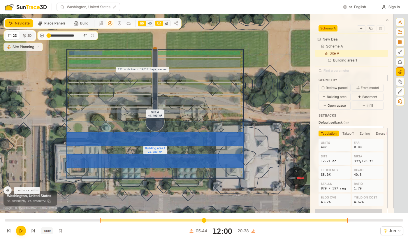
The guided start asks the four questions a feasibility study begins with, in the order they are usually answered, and ends on a solved scheme. It writes an ordinary document: everything it sets can be changed afterwards in the panel.
The four steps
- 1Where is it?Take the boundary from the extent of the loaded model, or draw it yourself on the ground. You cannot continue until there is a parcel.
- 2What is it zoned?Pick the closest district preset, or skip. Its rules are only checked; its setbacks change the design, so they are offered as a separate tick box.
- 3What are you building?Choose a typology and a number of floors, and whether to solve parking and circulation as well.
- 4What does it yield?The scheme is solved and its headline figures are shown: units, FAR, stalls and height. Open the full panel to refine it.
Sensible starting points
If the site has no unit mix yet, a typical four-type mix is added. When parking is requested, the lot is laid out as a band between the street frontage and the building, with room for the drive to turn, and a long frontage gets more than one way in.
Tip
Prefer to start from nothing? Choose Empty deal instead — the guided start is optional and never required.
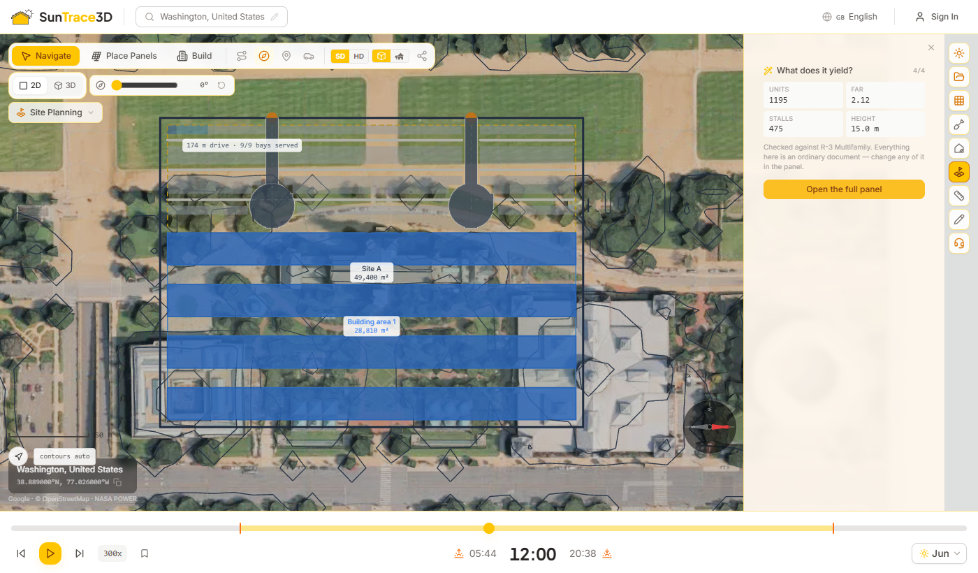
The parcel is the boundary everything else is measured from. Setbacks carve the buildable envelope out of it, and they are applied edge by edge.
Drawing the parcel
- 1Draw parcel or From modelChoose Draw parcel and click points on the ground, or From model to take the extent of the loaded model.
- 2Close the shapeClick the first point, double-click, or press Enter to close. Backspace removes the last point and Escape cancels.
- 3Set the setbacksEnter a default setback, then optional front, side and rear distances. A blank class field follows the default.
- 4Override single edgesThe edge list shows every parcel edge, how it was classified and the distance it actually received. Type a value against any edge to override it.
Automatic edge labels
Edges are classified as front, side or rear from the real streets around the site. An edge with no road near enough stays unclassified and takes the default.
Ignore roads and landscape buffer
Tick Ignore roads to treat every edge as the default. The landscape buffer adds a uniform band inside the setback line. Reset setbacks clears every override.
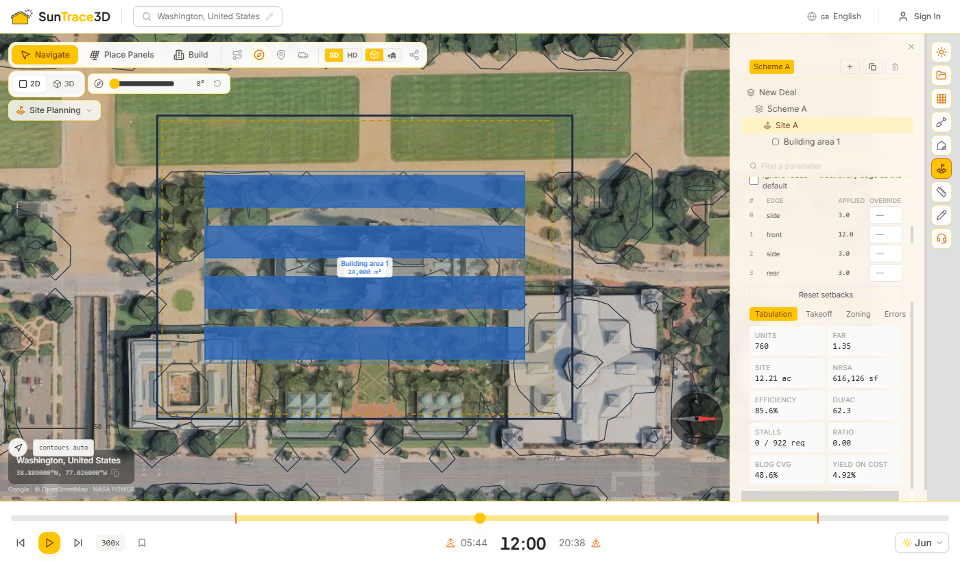
Regions divide the parcel into what gets built and what does not. Each region has a kind, and the solve treats each kind differently.
Region kinds
Building area
Ground a typology packs with buildings. Choose the typology for each building area in its properties.
Easement
Ground that must stay clear, such as a utility corridor. It is subtracted from the buildable envelope.
Open space
Parks, plazas and other ground kept free of buildings.
Infill
Builds only on the ground left over between buildings that are already solved — useful for filling gaps without overbuilding.
Pin
A pinned region keeps the parameters it was pinned with while the rest of the site follows the site settings.
Link
Linked regions of the same kind share their configuration, so a change to one applies to all. Their geometry always stays separate.
Schemes
Add, duplicate or delete schemes from the bar at the top of the panel. Each scheme is a complete, independent alternative.
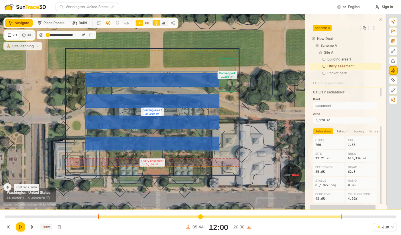
A typology is the rule set that turns a building area into buildings. Each family has its own logic rather than being one shape with different settings.
The six typologies
Double-loaded bar
Parallel residential bars with a central corridor, separated for light and air.
Residential over podium
Structured parking fills the base; homes sit on the deck above, set back from its edge.
Garden walk-up
A grid of small stair-served buildings with parking courts between them, limited to walk-up height.
Wrap around parking
A continuous band of homes on all four sides around a structured parking deck.
Industrial big box
One large warehouse sized after a truck court is reserved, reporting clear height and dock doors.
Data centre
Halls sized by power: reports IT capacity against your target load, and facility load at a chosen PUE.
Each family reports its own figures in the region properties — buildings and stairs for a walk-up, deck levels for a wrap, megawatts for a data centre.
Industrial and data centre schemes place no dwellings, so unit counts, density and residential parking demand read zero rather than an invented figure.
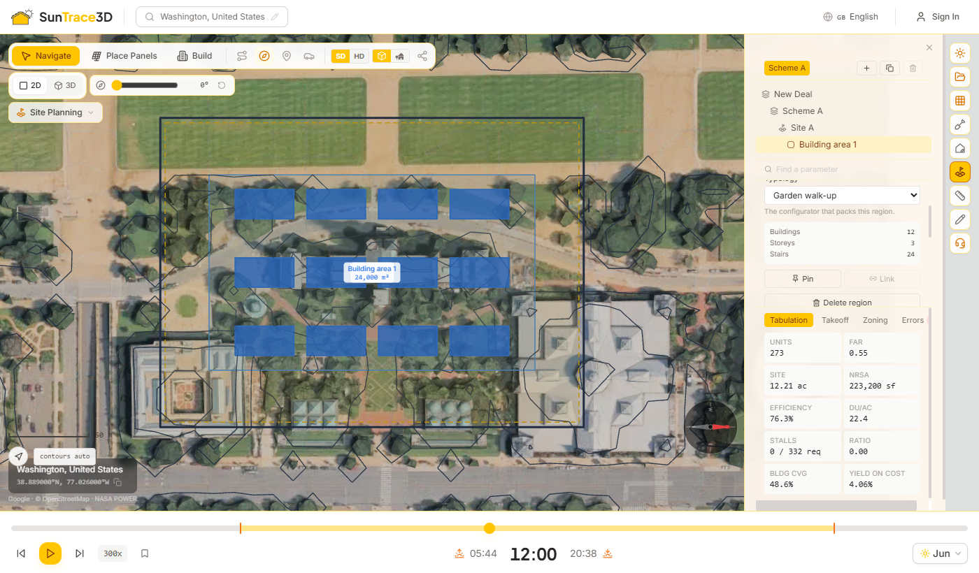
Unit mix and rates
In the Unit mix section, list the unit types with their share, target area and monthly rent, or start from a typical mix. In Rates, set land and build cost per m², rent per m² per year and cap rate. The pro forma is priced from the quantities the scheme actually solves to, so changing a setback moves the yield. Rates are indicative benchmarks.
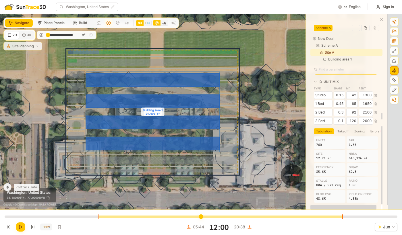
Parking and circulation are solved as part of the scheme. Parking fills the ground the buildings leave; circulation works out how a car reaches it from the street.
Parking
Turn on Solve parking to fill the remaining envelope with stalls and aisles. The bay direction is chosen for the most stalls, accessible stalls are added by the standard ratio, and you can switch between a surface lot, a structured deck and below-grade parking with a number of levels.
Circulation
Turn on Solve circulation. The drive enters from the frontage — the parcel edge nearest a road — through one or more curb cuts, runs into the site stopping short of buildings, and branches to the parking bays. A long dead end gets a turnaround.
Drives reserve their ground
The drive takes its space before parking is packed, so stalls are never drawn underneath the carriageway.
What it tells you
The readout shows the drive length, the paved area and how many bays are served. A bay the drive cannot reach is reported, not removed; a turnaround that does not fit is drawn in red.
Tip
Circulation is laid out as a spine with branches. On a very large site some bays may stay out of reach; add curb cuts or split the site into regions.
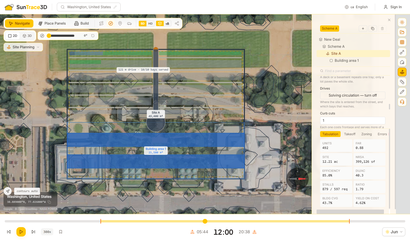
The results tabs under the panel show what the scheme yields and how it measures up. They update with every change.
Results tabs
Tabulation
Units, FAR, site area, net rentable area, efficiency, density, stalls provided against stalls required, parking ratio, coverage and yield on cost.
Takeoff
Quantities measured from the solved geometry — gross area, facade length, paving and stalls — priced into hard and total cost. Quantities are exact; costs use indicative rates.
Zoning
Every rule in the zoning profile by name, with its limit and a green or red chip for the value the scheme reached. Rules are checked only; a failing chip never changes the design.
Errors
Everything the solve wants you to know: parking shortfalls, unreachable bays, turnarounds that do not fit, a load the site cannot hold.
District presets
In step 2 or the Zoning tab, pick a district — single family, townhouse, multifamily, mixed use, commercial, industrial or data centre campus — to fill the checker in one step. A district also sets what the site builds: R-1 Single family fills the land with detached houses on their own plots, R-2 with terraces, R-3 with walk-ups, MU with a podium block, I-2 with a warehouse. The panel says so under the select, and step 3 can still change it. For houses, Homes are can be Mixed so each home type is detached, a semi-detached pair or a bungalow, and the Plot use bar shows how much of a plot is house, yard and garden. Its setbacks can be applied separately with Also apply its setbacks.
Presets are generic archetypes with typical North American values. They are a starting point, not your local code: replace them with the real zoning before relying on the result.
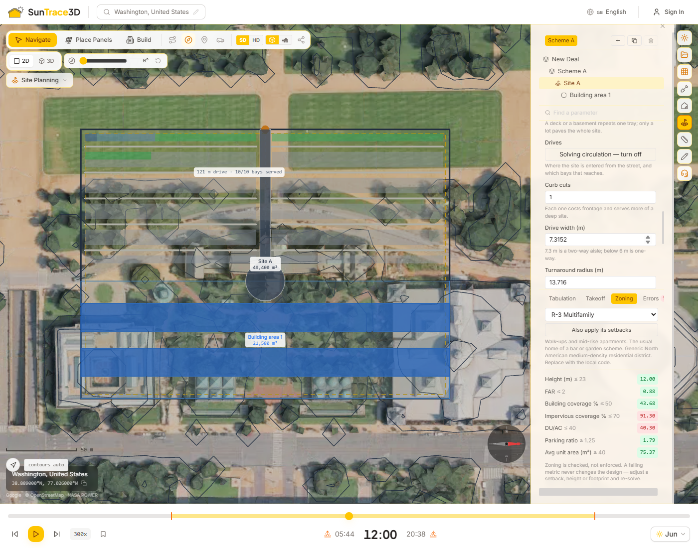
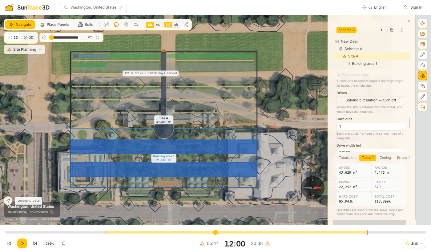
Once a scheme is solved, explore alternatives, bring in public site data, see it in 3D and take it into your own tools.
Generate options
Choose an objective — most units, highest FAR, best yield on cost, most parking or lowest cost — and run a sweep over floors, setbacks and stall angle. Options are ranked by that objective and each leads with the figure it was ranked by. Apply one to make it the live scheme.
Data layers
Fetch free public layers for the parcel: FEMA flood hazard, utilities and wetlands from OpenStreetMap. High-risk flood zones and wetlands can be added to the site as easements in one click.
See it in 3D
Switch to 3D to see the solved buildings extruded to their height, standing on the real ground of the model among the existing city.
Export
Download the plan as DXF for CAD, with parcel, envelope, buildings and parking on named layers; as SVG for documents; and the takeoff as CSV.
Flood data covers the USA only, and the FEMA service may refuse connections from outside the USA. OpenStreetMap coverage of utilities and wetlands varies by area. A layer marked unavailable means its service could not be reached; a count of 0 means it answered and found nothing.
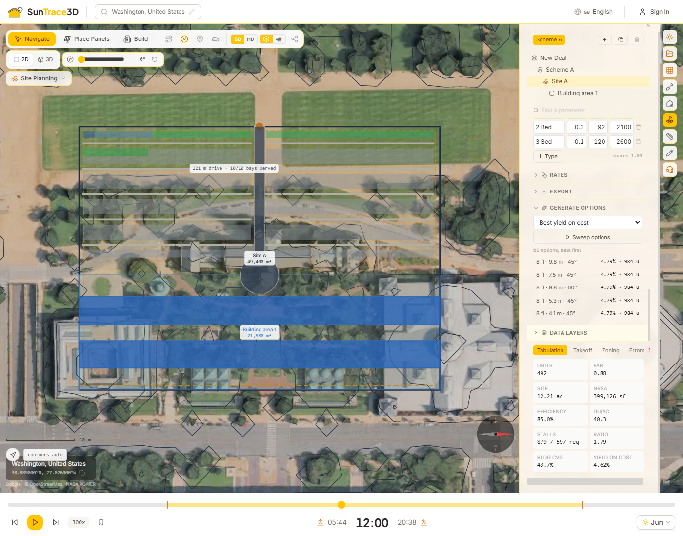
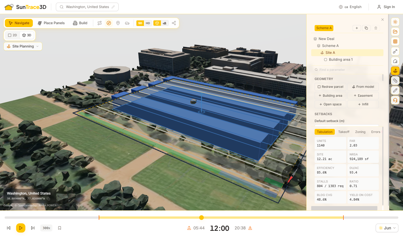
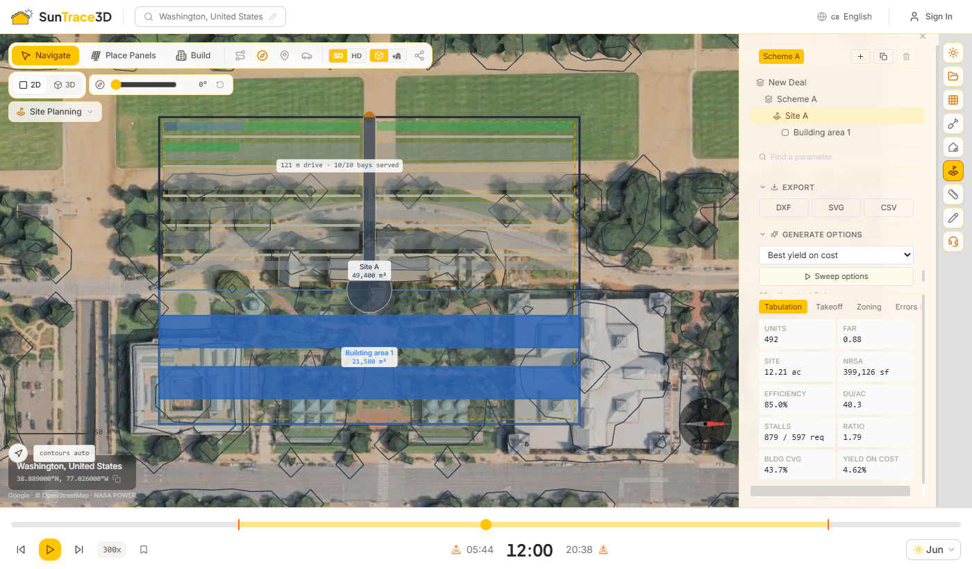
Undo and redo any action, select multiple objects at once, and copy/paste them — all with familiar keyboard shortcuts. These tools work across solar panels, scene objects (trees, fences, pergolas, etc.), buildings, and measurements.
Undo & Redo
Press Ctrl+Z to undo your last action, or Ctrl+Y to redo it. Every placement, deletion, move, rotation, and property change is tracked. The undo history supports batch operations — for example, the Solar Wizard's panel placement can be undone in one step.
Multi-Select
Hold Shift and click on panels or scene objects to add or remove them from your selection. Selected items are highlighted in blue. You can Shift+click in both Navigate and Build modes.
Copy & Paste
With one or more items selected, press Ctrl+C to copy and Ctrl+V to paste. Pasted items appear offset to the right. You can paste multiple times — each paste offsets further. This works for both solar panels and scene objects.
Batch Delete
Select multiple items with Shift+click, then press Delete to remove them all at once. The deletion can be undone with Ctrl+Z.
Tip
Undo and redo work across all object types — panels, buildings, scene objects, and measurements. If you undo a wizard placement, all panels placed by the wizard are removed in one step.
The Weather Forecast panel predicts what your system will actually produce over the next 7 days, using the real hourly weather forecast for your location instead of long-term averages. It reuses the same irradiance and shading model as the annual yield figures, then adds the short-horizon effects that only matter week to week: cloud cover, cell heating, dust build-up between rain events, snow cover and inverter clipping.
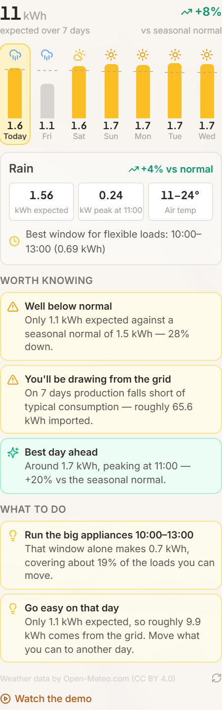
How to use it
- 1Place your panelsThe forecast runs against the layout currently in the scene — real tilts, real azimuths and the per-panel shading losses the shadow analysis already calculated. Change a panel and the forecast updates immediately.
- 2Open Solar Analysis → Weather ForecastThe bar chart shows expected production per day. The dashed line on each bar is the seasonal normal for that date and location, so you can see at a glance whether a day is running ahead of or behind what is typical.
- 3Tap a day for the detailEach day expands to show expected kWh, peak power and the hour it occurs, the temperature range, the best window for running flexible loads, and a breakdown of what heat, soiling and clipping cost you that day.
Real hourly weather
Hourly global, direct and diffuse irradiance, air temperature, wind, rain and snow come from Open-Meteo and are transposed onto each panel's own plane. Wind cooling and cell heating are modelled explicitly, because a hot still day and a hot breezy day do not produce the same amount.
Compared to seasonal normal
Every day is measured against the 22-year NASA POWER climatology for your exact location — the same baseline behind the annual yield figure. That is what makes "18% below normal" meaningful rather than just a number.
Anomaly alerts
The forecast flags what is worth knowing: snow that will cover the array, a multi-day slump, heat that is quietly costing several percent, storm-force wind worth a mounting check, inverter clipping, and rain that will clean the panels for free.
Day-by-day advice
Alerts turn into actions: the best three-hour window for the washing machine or EV charger, which day to pre-charge the battery, which day to go easy because you will be importing, and when clearing snow is worth the trip up.
What the numbers mean
Expected production is the AC energy after shading, balance-of-system losses, temperature derate, soiling, snow cover and inverter clipping. The clear-sky ceiling is the same system under a cloudless sky, and the seasonal normal is that ceiling scaled by the local climatological clear-sky index. A day well above normal is a genuinely clear day; a day well below it is one to plan around.
Plan availability
The weather forecast is available on all paid plans. Personal covers 7 days, Business 14 days and Enterprise 16 days. Free accounts receive a weekly summary for their area in the newsletter instead.
Tip
The seasonal-normal line is the useful one. A cloudy week in June still out-produces a bright week in December, so raw kWh alone will not tell you whether something is wrong. If a day reads far below normal and the weather does not explain it, check the shading analysis — that is usually where the answer is.
Download everything in the scene as a single 3D file and carry on in the tool you already use. The export contains the generated terrain and buildings, every solar panel you placed, ground-mount arrays with their posts, custom and detected buildings, placed objects such as trees and fences, and any model you imported — in the same positions and orientations you see in the viewer. Included in the Business plan and above.
How to export
- 1Open the Projects panelLoad a location and build your design as usual. The Export scene block sits at the bottom of the Projects panel in the sidebar.
- 2Choose GLB or OBJGLB is one binary file with textures and materials — it opens directly in Blender, SketchUp, Rhino, Unity, Unreal, Three.js viewers and most CAD packages. OBJ is geometry only, with no textures, for older tools that cannot read GLB.
- 3DownloadThe file is built in your browser from the live scene, so whatever is on screen at that moment is what you get — including changes you have not saved yet. Large HD models can take a few seconds.
What is in the file
Named groups keep the layers apart: Terrain, Buildings, SceneObjects, ImportedModels, GroundMountStructure and SolarPanels, with each panel as its own mesh. Editing helpers — selection outlines, drag handles, the sun path, heatmaps — are never exported.
Units and orientation
Metres, Y up, with +X east and +Z south, matching the viewer. The origin is the centre of the generated model, not a geographic coordinate, so combine the export with the project location if you need to georeference it.
Plan availability
Scene export is part of the Business and Enterprise plans. Free and Personal accounts see the option in the Projects panel and can upgrade from there.
Export after you save. The download reflects the scene exactly as it is on screen, so saving first means the file and the project match, and a colleague opening either sees the same design.
The Weather Forecast panel tells you about the week ahead while you are in the app. The weekly forecast brings it to you instead. Once a week you get the same numbers for your own roof — by email, by browser notification, or both — so a bad week does not surprise you and a good one does not go unused.
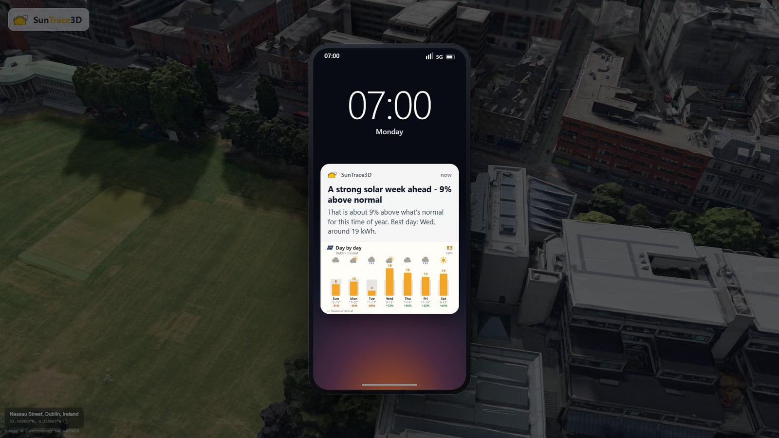
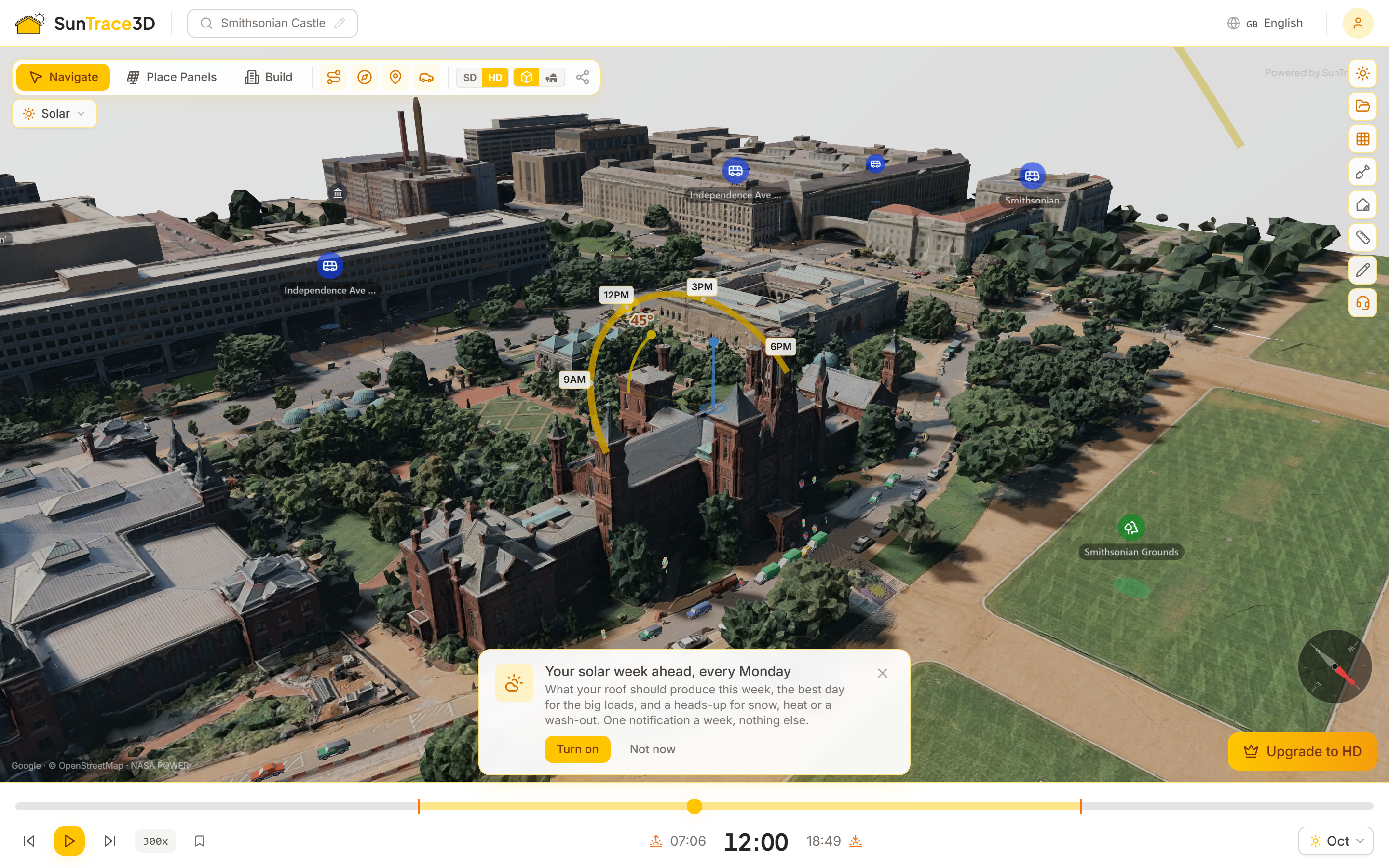
Turning it on
- 1Accept the offer, or use Account → PreferencesA small card offers browser notifications once you are signed in. You can also turn either channel on at any time under Account → Preferences. The email is on by default; notifications are always opt-in.
- 2Give us a roof to forecastThe forecast is for a real place: a saved project, a model you generated, or a location you looked at. Demo locations and landmarks are never used, so nobody receives a forecast for somewhere they have never been.
- 3Open it and land on your roofClicking the email or the notification opens the viewer on your own project with the forecast panel already open. Without a saved layout it opens your location with a card repeating the week you were just sent.

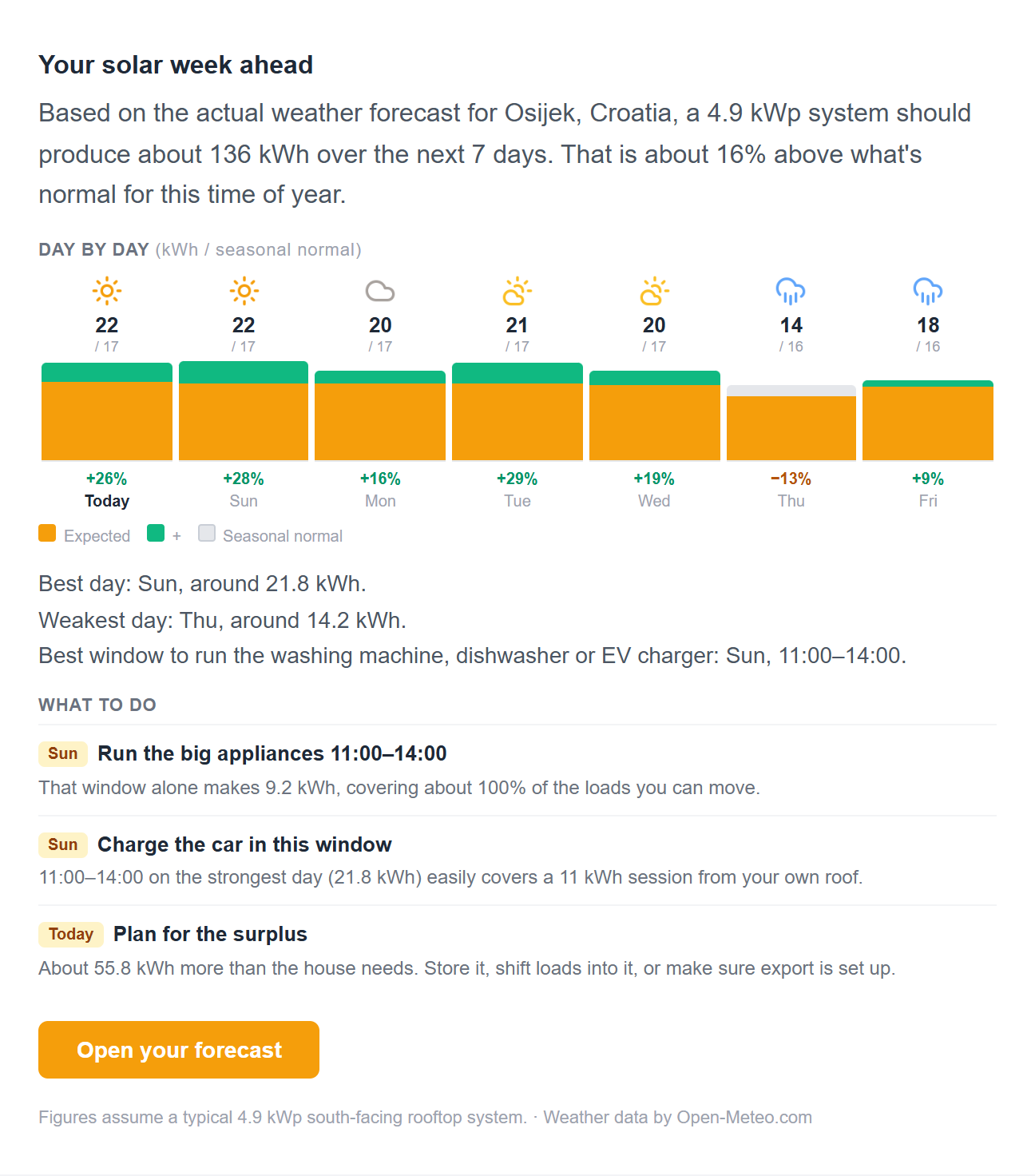
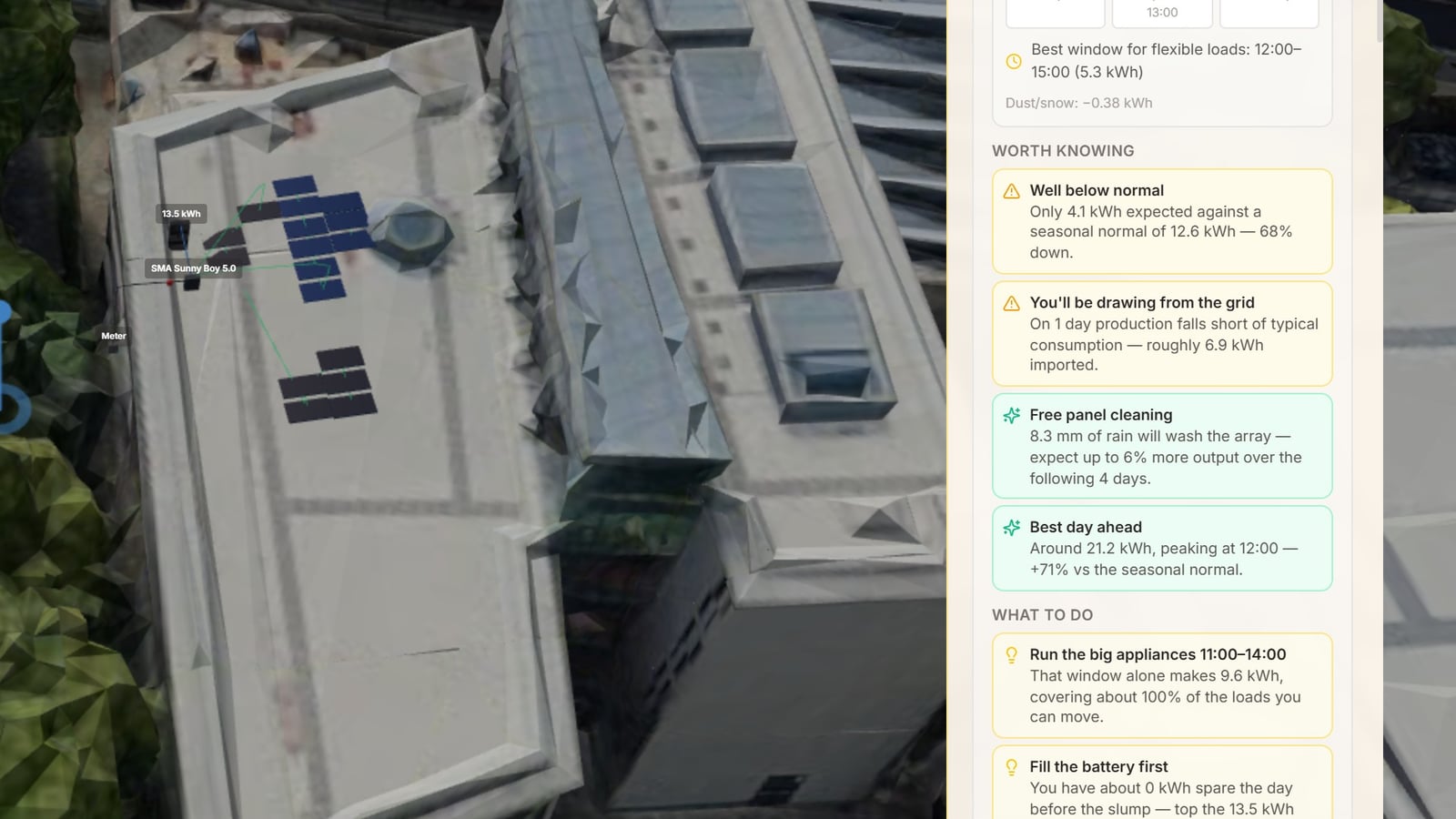
The email
The week against the seasonal normal, a bar for each day, the best day, the weakest day, the best window for the washing machine or the car, and up to four things worth doing. Subscribers see their own saved layout; everyone else sees a reference rooftop for their location.
The browser notification
One notification a week, with the week's verdict and the best day. Tapping it opens the same place the email does. It works on desktop and Android browsers; on Chrome it also carries a picture of the week.
Sent when you are actually around
Not a fixed Monday morning for everyone. The send time is learned from when you use the app and open mail, in your own time zone, and never lands in the middle of the night.
It stops if you stop reading
Ignore four in a row and it drops to monthly. Ignore seven and it pauses entirely until you use the app again. Opening one, clicking one, or simply coming back resets it. You will not be nagged.
iPhone and iPad
Safari only delivers notifications to an installed app, so add SunTrace3D to your Home Screen first, then turn notifications on from there. Until you do, the email covers you. Apple does not show a picture on web notifications.
Who gets what
Everyone with an account and a real location can receive the weekly forecast. Subscribers get it for their own saved system; free accounts get it for a reference rooftop at the same place, with the full detail behind the upgrade.
Tip
If you want it only as a notification, turn the email digest off under Account → Preferences. The two channels are independent, and stopping the weekly email never affects anything else we send you.
Building an integration?
Check out the API documentation for generating models programmatically and embedding 3D views on your website.
API DocumentationOn This Page
Getting Started
1.Getting Started- 2.3D Navigation Controls
- 3.Searching for Locations
Sun & Shadows
4.Shadow Simulation- 5.Sun Path Visualization
Solar Panels
6.Solar Panel Placement- 7.Shadow Analysis
- 8.Energy Yield Analysis
- 33.Solar Wizard
- 34.Ground Mount Arrays
- 45.Panel Irradiance Heatmap
- 71.Weather Forecast
- 73.Weekly Forecast by Email and Notification
Quality & Views
9.SD & HD Quality Modes- 10.Compass & Orientation
- 23.Standard & Realistic Models
- 52.Ambient Life
- 54.Plan Mode (2D)
Build Mode
11.Building Placement- 12.Scene Objects & Landscaping
- 13.Bulldozer Tool
- 51.Draw a House
Garden & Heatmap
14.Sunlight Heatmap- 15.Garden Planner
Analysis & Reports
16.Climate Data- 17.Installation Cost & Get Quote
- 18.Solar Impact
- 19.Site Report
- 46.Loss Waterfall Chart
- 49.PDF Quotes
Tools & Navigation
20.Keyboard Shortcuts- 21.Measurement Tool
- 22.Points of Interest
- 35.Draw Tool
- 50.Undo, Redo & Multi-Select
Account & Projects
24.Account & Subscription- 25.Project Management
- 26.Importing 3D Models
- 36.3D Model Library
- 53.Share for Review
- 63.Team Workspace
- 64.Branded Proposals
- 65.Electronic Signature
- 66.From Feedback to Signature
- 72.Export the 3D Scene
Engineering & Design
37.Module & Inverter Catalog- 38.String Planning
- 39.Single-Line Diagram
- 40.Cable Sizing
- 41.Self-Consumption Analysis
- 42.Battery Storage
- 47.Energy System Dashboard
- 43.Bill of Materials
- 44.PVsyst Export
Industry Verticals
27.Right-to-Light Compliance- 28.Urban Heat Analysis
- 29.Film & Photography Tools
- 30.Real Estate Analysis
- 31.Agriculture & Crop Planning
- 32.Live Events & Outdoor Hospitality
- 48.CRM Platform
- 67.From Prospect to Signed Deal
Regulatory
68.German Regulatory Pack- 69.Grid Compliance Pre-Check
- 70.Tenant Electricity (Mieterstrom)
Site Planning
55.Site Planning Overview- 56.Guided Start
- 57.Parcel & Setbacks
- 58.Regions & Schemes
- 59.Typologies & Unit Mix
- 60.Parking & Circulation
- 61.Zoning & Results
- 62.Options, Data Layers & Export